A 2nd, better way to WorldCupGraph

Hours after publishing my previous blogpost about the WorldCup Graph, I actually found a better, and more up to date dataset that contained all the data of the actual squads that are going to play in the actual World Cup in Qatar. I found it on this wikipedia page, which lists all the tables with the actual squads, some player details, coaches etc. as they were announced on 10th/11th of November.

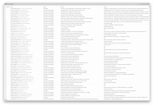
So: I figured it would be nice to revisit the WorldcupGraph, and show a simpler and faster way to achieve the results of the previous exercise. So: I have actually put this data in this spreadsheet, and then downloaded a .csv version:

• one .csv file containing the squads
• one .csv file containing the tournament schedule (just like in the previous example, actually)

These two files are super nice and simple, and therefore we can actually use the Neo4j Data Importer toolset to import these really easily.

No WorldCup without a WorldCupGraph!

Last week I was having a conversation with one of my dear Neo4j colleagues, and we were talking about the fact that Graphs are simply so much fun to play around with, and that there's nothing like a great interesting dataset to have people really experiment and acquaint themselves with the technology. I know that to be extremely true, and I think I have demonstrated this elaborately over the years on this runaway blog of mine.

Then the conversation turned to a topic that I know very little about: the FIFA World Cup in Qatar that is starting next week. Now, reading this blog you may know that I am a little addicated to my 2 wheeled #mentalhealthmachine, and that chasing a ball across a field seems like a little bit of a game to me - but hey, that's ok! And with this conversation it actually dawned on me that at Neo4j, we had done "Worldcup Graphs" both in 2014 and in 2018: our friend and former colleague Mark Needham was the driving force behind both of those efforts.

You can still see some of the work that Mark did at the time on Github and Medium. It was truly another example of how a cool and timely dataset would get people to explore the wonderful world of graphs and get to know the technology in a fun and interesting way.

So: I decide that it would be nice to do that again. With all the new tech that is coming out of Neo4j with the release of Neo4j 5, that could not be very difficult, right? Let's take a look.

A Graph Database and a Dadjoke walk into a bar...

I just publised a blogpost series with 6 different articles about me having fun with Dadjokes, in an unusual sort of way. Here are the links to the articles:

• Part 1/6: Building a Dadjoke database - from nothing
• Part 2/6: Importing the Dadjokes into the Dadjoke Graph
• Part 3/6: Taking on the real disambiguation of the jokes
• Part 4/6: Adding NLP and Entity Extraction to prepare for further disambiguation
• Part 5/6: Disambiguation using Graph Data Science on the NLP-based Entities
• Part 6/6: Closing: some cool Dadjoke Queries

All of the queries etc are put together in this markdown document. I plan to make a Neo4j Guide out of this as well in the next few days so that it would become easier to use. 

Hope you will have as much fun with it as I did. 

Rik

• Twitter
• Blog
• LinkedIn

DadjokeGraph Part 6/6: Closing: some cool Dadjoke Queries

A Graph Database and a Dadjoke walk into a bar...

Now that we have a disambiguated graph of dadjokes, let's have some fun and explore it.

How many times does a joke get tweeted?

MATCH ()-[r:REFERENCES_DADJOKE]->(dj:Dadjoke)
WITH dj.Text AS Joke, count(r) AS NrOfTimesTweeted
RETURN Joke, NrOfTimesTweeted
ORDER BY NrOfTimesTweeted DESC
LIMIT 10;

How many times does a joke get favorited?

MATCH ()-[r:REFERENCES_DADJOKE]->(dj:Dadjoke)
RETURN dj.Text AS Joke, dj.SumOfFavorites AS NrOfTimesFavorited, dj.SumOfRetweets AS NrOfTimesRetweeted
ORDER BY NrOfTimesFavorited DESC
LIMIT 10;

DadjokeGraph Part 2/6: Importing the Dadjokes into the Dadjoke Graph

A Graph Database and a Dadjoke walk into a bar...

This means that we want to convert the spreadsheet that we created before, or the .csv version of it, into a Neo4j Database.

Here's how we go about this. First things first: let's set up the indexes that we will need later on in this process:

CREATE INDEX tweet_index FOR (t:Tweet) ON t.Text;
CREATE INDEX dadjoke_index for (d:Dadjoke) ON d.Text;

Assuming the .csv file mentioned above is in the import directory of the Neo4j server, we can use load csv to create the initial dataset:

LOAD CSV WITH HEADERS FROM "file:/vicinitas_alldadjokes_user_tweets.csv" AS csv
CREATE (t:Tweet)
SET t = csv;

Or: if you want to create the graph straight from the Google Sheet:

LOAD CSV WITH HEADERS FROM "https://docs.google.com/spreadsheets/d/1MwHX5hM-Vda5o4ZQVnCv4upKepL5rHxcUrqfT69u5Ro/export?format=csv&gid=1582640786" AS csv
CREATE (t:Tweet)
SET t = csv;

DadjokeGraph Part 3/6: Taking on the real disambiguation of the jokes

A Graph Database and a Dadjoke walk into a bar...

We noticed that many of the Tweet nodes referred to the same jokes - and resolved that already above. But this query makes us understand that we actually still have some work to do:

MATCH path = (dj:Dadjoke)-[*..2]-(conn)
WHERE dj.Text CONTAINS "pyjamazon"
    RETURN path;

We will come back to that example below.

We now notice that there are quite a few Dadjoke nodes that are a bit different, but very similar. We would like to disambiguate these too. We will use a couple of different strategies for this, but start with a strategy that is based on String Metrics.

DadjokeGraph Part 4/6: Adding NLP and Entity Extraction to prepare for further disambiguation

A Graph Database and a Dadjoke walk into a bar...

As we can see in the pyjamazon example from before, the disambiguation of our Dadjokes has come a long way - but is not yet complete. Hence we we call the graph to the rescue here, and take it a final step further that will provide a wonderfully powerful example of how and why graphs are so good at analysing the structural characteristics of data, and make interesting and amazing recommendations on the back of that.

Here's what we are going to do:

1. we are going to use Natural Language Processing to extract the entities that are mentioned in our Dadjokes. Do do that, we are going to use the amazing Google Cloud NLP Service, and call it from APOC. This will yield a connected structure that will tell us exactly which entities are mentioned in every joke.
2. then we are going to use that graph of dadjokes connected to entities to figure out if the structure of the links can help us with further disambiguation of the jokes.

So let's start with the start.

DadjokeGraph Part 5/6: Disambiguation using Graph Data Science on the NLP-based Entities

A Graph Database and a Dadjoke walk into a bar...

The next, and final, step our dadjoke journey here, is going to be taking the disambiguation to the next level by applying Graph Data Science metrics to the new, enriched (using NLP), structure that we have in our graph database. The basic idea here is that, while the TEXT similarity of these jokes may be quite far apart, their structural similarity may still be quite high based on the connectivity between the joke and its (NLP based) entities.

Calculating the Jaccard similarity metric using GDS

To explore this, we will be using the Jaccard similarity coefficient, which is part of the Neo4j Graph Data Science library that we have installed on our server. More about this coefficient can be found on Wikipedia. The index is defined as the size of the intersection divided by the size of the union of the sample sets, which is very well illustrated on that Wikipedia page. I have used Neuler (the no-code graph data science playground that you can easily add to your Neo4j Desktop installation) to generate the code below - but you can easily run this in the Neo4j Browser as well.

DadjokeGraph Part 1/6: Building a Dadjoke database - from nothing

A Graph Database and a Dadjoke walk into a bar...

I am a dad. Happily married and 3 wonderful kids of 13, 17 and 19 years old. So all teenagers - with all the positive and not so positive experiences that can come with that. And in our family, I have been accused of using dadjokes - preferably at very awkward or inconvenient times. I actually like dadjokes. A lot.

So I follow a few accounts on social media that post these jokes. Like for example baddadjokes, dadjokeman, dadsaysjokes, dadsjokes, groanbot, punsandoneliner, randomjokesio, and thepunnyworld and there are many others. These are all in this list, should you be interest. It's a very funny list.

Graphs are everywhere - also in Religious Texts - part 6 and close - Analysing the Hadith Narrator Graph

So what we will do here, is we will start looking at some of the structural graph metrics that are going to give us a little bit more insight into the importance of different parts of the Hadith Narrator Graph. We will use the Neuler Graph Data Science playground to do that. Neuler is a so-called GraphApp that you can easily install into your Neo4j Desktop environment. You can download and install it, and learn more about it here.

Once installed, we will run a few easy algo's.

Pagerank centrality of the Scholars

Once of the advantages of the AGGREGATED_HADITH_CHAIN relationship, is that we now have a mono-partite, weighted subgraph that is very suitable for understanding which Scholars are actually more interesting than others - this is a great use case for the Pagerank algorithm. Here's how we configure it:

Graphs are everywhere - also in Religious Texts - part 5 - Exploring the Hadith Narrator Graph

Before we can start that exploration, we do need to put in place a few additional indexes that have not yet been created in the import process: on the english translations of the hadiths, and on the scholar names. That's simple operation:

CREATE TEXT INDEX hadith_text_en FOR (h:Hadith) ON (h.text_en);
CREATE TEXT INDEX scholar_name FOR (s:Scholar) ON (s.name);

Note that these indexes are not full text indexes - but they are more optimised for text fields.

The model now looks like this: 

So now we can start some querying. This query gives us a flavour of what we could find:

MATCH (:Scholar)--(n:Hadith)--(:Source)
RETURN n LIMIT 25;

Graphs are everywhere - also in Religious Texts - part 4 - Connect the Hadiths with the scholars

Now, we will connect the Hadiths with the scholars:

:auto MATCH (h:Hadith)
WITH h, split(replace(h.chain_indx," ",""),",") as scholarlist
CALL
    {
    WITH h, scholarlist
    UNWIND scholarlist as scholar
        MATCH (s:Scholar {scholar_indx: scholar})
        MERGE (s)-[:NARRATED]->(h)
    } IN TRANSACTIONS OF 100 ROWS;

Graphs are everywhere - also in Religious Texts - part 3 - Importing the Hadiths into Neo4j

Again, just like in part 2, we will use the Neo4j Data Importer for this. You can find the .zip file with the model and the dataset over here. In this operation we actually first create a separate subgraph for the Hadiths and the sources:

 This operation returns very quickly:  And offers a good view of the result: 

Graphs are everywhere - also in Religious Texts - part 2 - import the Hadith narrators into Neo4j

The source data that we found in part 1 is in a .csv format - so that means that it basically looks tabular:

Luckily, we nowadays have some fantastic tools to import these files, without writing any code at all using the all new Neo4j Data Importer. After drawing a few nodes and relationships, I was able to do the basic import:  It was super quick to return after a few seconds: 

Graphs are everywhere - also in Religious Texts - part 1 - Introduction

This is going to be an interesting and in some ways even fascinating set of blogposts. I have thoroughly enjoyed researching it and playing around with the latest and greates Neo4j tools while doing so, but I must say that it's also one of the first blogposts that I can remember where I am a bit uneasy about the content. Why? Because it's about, or at least in some ways touches, religion.

First let's start with some background here. Some things that you should know about me:

• I was born and raised in Belgium, which is - or at least was - a predominantly Catholic Christian country. There's churches and chapels on every corner of the street here.
• My parents were/are far from religious, never took me to church, but did give me many of the Catholic Christian values - and these were engrained in me even more clearly because of my 13 ears in Jesuit schools in Antwerp and Turnhout.
• as an adult, I became increasingly distantiated from all religious beliefs. In my twenties and thirties I was still a "cultural Christian", I guess, as exemplified by the fact that we got married in church, and baptised all of our 3 children. In my late thirties and forties, ie. now, I becaome convinced that not much good can come of religion - in general. I read Richard Dawkins, Christopher Hitchens, Sam Harris, and similar authors that have a very sceptic, atheist view on religion. And I like it that way, for me, personally.
• that personal choice does not mean that I have something against people that still have a faith. I am totally fine with anyone believing what they want to believe - as longs as they don't hurt others or impose on others during the process.

But, and here's the sensitive bit: this blogpost will be about Islam - and Moslim holy books and texts very specifically. There's no reason for me choosing to write about this specific religion - other than the fact that it came across my path and I thought some of the material was absolutely fascinating.

Conway's Game of Life in Neo4j

A couple of weeks ago, me and my Neo4j Breakfast Club friends were just freewheeling our way into the day, and one of my colleagues started talking to me about Conway's Game of Life.. I had never heard of this thing, but was immediately fascinated. It basically allows you to simulate evolution in a rudimentary and simplified kind of way, but it's really fascinating how it works based on a very simple set of rules (see below). There's an entire Wiki dedicated just to this "game" - it's one of the most wonderful rabbitholes on the web that I have ever seen. Just take a look at this example and you will see the idea in action:

The Game of Life, also known simply as Life, is a cellular automaton devised by the British mathematician John Horton Conway in 1970. It is a zero-player game, meaning that its evolution is determined by its initial state, requiring no further input. One interacts with the Game of Life by creating an initial configuration and observing how it evolves. It is Turing complete and can simulate a universal constructor or any other Turing machine.

So when I heard about it, I immediately thought that it would be a ton of fun to run this experiment in Neo4j. Why? Because the rules are all about connections between members of a population. Things will evolve - or not - based on their connectivity.

Importing (BEER) data into Neo4j - WITHOUT CODING!

Importing data into a graph structure stored in a graph database can be a real pain. Always has been, probably always will be to some degree. But we can really make the pain be a lot more tolerable - and today's blogpost is going to be about just that. The reason for this is pretty great: Neo4j has just launched a new online tool that allowed me to make the whole process a really easy and straightforward experience - take a look at it at http://data-importer.graphapp.io.

So let me try to explain how it works in the next few paragraphs.

First: find a dataset

Obviously the internet is flooded with data these days - but for this exercise I used https://datasetsearch.research.google.com/ for the first time. Amazing tool, as usual from Google. And I quickly found an interesting one that I could download from Kaggle.

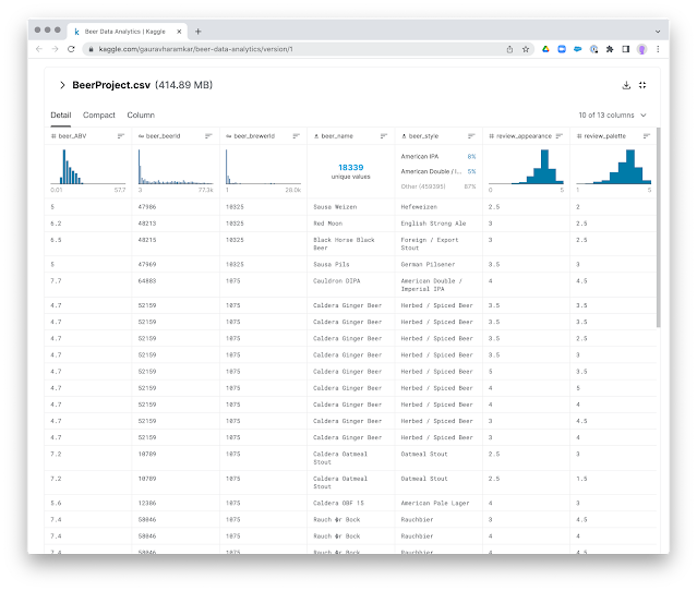
This dataset contains information about the different types of beers and various aspects of it such beer style, absolute beer volume, beer name, brewer name, beer appearance, beer taste, its aroma, overall ratings, review, etc.  - and it does so in a single .csv file with about 500k rows. Cool. 

So I was ready to take that to the importer.