The Great Olympian Graph - part 2/3

In the previous blogpost of this Olympic series I explained how I got to the dataset in 4 distinct .csv files that get generated from a 4-worksheet Google Spreadsheet. Here are the links to the 4 sheets:

• The Countries sheet, including the country codes
• The Cities sheet, mapped to the countries
• The Sports Taxonomy sheet, with the sports and disciplines
• and finally: The Medallists sheet.

Now, in order to load that data into Neo4j, I had to come up with a meaningful graph model.

The GraphBlogGraph: 2nd blogpost out of 3

Importing the GraphBlogGraph into Neo4j

In the previous part of this blog-series about the GraphBlogGraph, I talked a lot about creating the dataset for creating what I wanted: a graph of blogs about graphs. I was able to read the blog-feeds of several cool graphblogs with a Google spreadsheet function called “ImportFEED”, and scrape their pages using another function using “ImportXML”. So now I have the sheet ready to go, and we also know that with a Google spreadsheet, it is really easy to download that as a CSV file:

You then basically get a URL for the CSV file (from your browser’s download history):

and that gets you ready to start working with the CSV file:

I can work with that CSV file in Cypher’s LOAD CSV command, as we know. All we really need is to come up with a solid Graph Model to do what we want to do. So I went to Alistair’s Arrows, and drew out a very simple graph model:

So that basically get’s me ready to start working with the CSV files in Cypher. Let’s run through the different import commands that I ran to do the imports. All of those are on github of course, but I will take you through them here too...

First create the indexes

create index on :Blog(name);

create constraint on (p:Page) assert p.url is unique;

Then manually create the blog-nodes:

create (b:Blog {name:"Bruggen", url:"http://blog.bruggen.com"});

create (n:Blog {name:"Neo4j Blog", url:"http://neo4j.com/blog"});

create (n:Blog {name:"JEXP Blog", url:"http://jexp.de/blog/"});

create (n:Blog {name:"Armbruster-IT Blog", url:"http://blog.armbruster-it.de/"});

create (n:Blog {name:"Max De Marzi's Blog", url:"http://maxdemarzi.com/"});

create (n:Blog {name:"Will Lyon's Blog", url:"http://lyonwj.com/"});

I could have done that from a CSV file as well, of course. But hey - I have no excuse - I was lazy :) … Again…

Then I can start with importing the pages and links for the first (my own) blog, which is at blog.bruggen.com and has a feed at blog.bruggen.com/feeds/posts/default:

//create the Bruggen blog entries

load csv with headers from "https://docs.google.com/a/neotechnology.com/spreadsheets/d/1LAQarqQ-id74-zxV6R4SdG7mCq_24xACXO5WNOP-2_w/export?format=csv&id=1LAQarqQ-id74-zxV6R4SdG7mCq_24xACXO5WNOP-2_w&gid=0" as csv

match (b:Blog {name:"Bruggen", url:"http://blog.bruggen.com"})

create (p:Page {url: csv.URL, title: csv.Title, created: csv.Date})-[:PART_OF]->(b);

This just creates the 20 leaf nodes from the Blog node. The fancy styff happens next, when I then read from the “Links” column, holding the “****”-separated links to other pages, split them up into individual links, and merge the pages and create the links to them. I use some fancy Cypher magic that I have also used before for Graph Karaoke: I read the cell, and then split the cell into parts and put them into a collection, and then unwind the collection and iterate through it using an index:

//create the link graph

load csv with headers from "https://docs.google.com/a/neotechnology.com/spreadsheets/d/1LAQarqQ-id74-zxV6R4SdG7mCq_24xACXO5WNOP-2_w/export?format=csv&id=1LAQarqQ-id74-zxV6R4SdG7mCq_24xACXO5WNOP-2_w&gid=0" as csv

with csv.URL as URL, csv.Links as row

unwind row as linklist

with URL, [l in split(linklist,"****") | trim(l)] as links

unwind range(0,size(links)-2) as idx

MERGE (l:Page {url:links[idx]})

WITH l, URL

MATCH (p:Page {url: URL})

MERGE (p)-[:LINKS_TO]->(l);

So this first MERGEs the new pages (finds them if they already exist, creates them if they do not yet exist) and then MERGEs the links to those pages. This creates a LOT of pages and links, because of course - like with every blog - there’s a lot of hyperlinks that are the same on every page of the blog (essentially the “template” links that are used over and over again).

And as you can see it looks a little bit like a hairball when you look at it in the Neo4j Browser:

So in order to make the rest of our GraphBlogGraph explorations a bit more interesting, I decided that it would be useful to do a bit of cleanup on this graph. I wrote a couple of Cypher queries that remove the “uninteresting”, redundant links from the Graph:

//remove the redundant links

//linking to pages with same url (eg. archive pages, label pages...)

match (b:Blog {name:"Bruggen"})<-[:PART_OF]-(p1:Page)-[:LINKS_TO]->(p2:Page)

where p2.url starts with "http://blog.bruggen.com"

and not ((b)<-[:PART_OF]-(p2))

detach delete p2;

//linking to other posts of the same blog

match (p1:Page)-[:PART_OF]->(b:Blog {name:"Bruggen"})<-[:PART_OF]-(p2:Page),

(p1)-[lt:LINKS_TO]-(p2)

delete lt;

//linking to itself

match (p1:Page)-[:PART_OF]->(b:Blog {name:"Bruggen"}),

(p1)-[lt:LINKS_TO]-(p1)

delete lt;

//linking to the blog provider (Blogger)

match (p:Page)

where p.url contains "//www.blogger.com"

detach delete p;

Which turned out to be pretty effective. When I run these queries I weed out a lot of “not so very useful” links between nodes in the graph.

And the cleaned-up store looks a lot better and workable.

If you take a look at the import script on github, you will see that there’s a similar script like the one above for every one of the blogs that we set out to import. Copy and paste that into the browser one by one, the neo4j shell, or use LazyWebCypher, and have fun:

So that’s it for the import part. Now there’s only one thing left to do, in Part 3/3 of this blogpost series, and that is to start playing around with some cool queries. Look that post in the next few days.

Hope this was interesting for you.

Cheers

Rik

Querying GTFS data - using Neo4j 2.3 - part 2/2

So let's see what we can do with this data that we loaded into Neo4j in the previous blogpost. In these query examples, I will try to illustrate some of the key differences between older versions of Neo4j, and the newer, shinier Neo4j 2.3. There's a bunch of new features in that wonderful release, and some of these we will illustrate using the (Belgian) GTFS dataset. Basically there's two interesting ones that I really like:

• using simple "full-text" indexing with the "starts with" where clause
• using ranges in your where clauses

Both of these were formerly very cumbersome, and very easy and powerful in Neo4j 2.3. So let's explore.

Finding a stop using "STARTS WITH"

In this first set of queries we will be using some of the newer functionalities in Neo4j 2.3, which allow you to use the underlying full-text search capabilities of Lucene to quickly and efficiently find starting points for your traversals. The first examples start with the "START WITH" string matching function - let's consider this query:

 match (s:Stop)  
 where s.name starts with "Turn"  
 return s  

In the new shiny 2.3 version of Neo4j, we generate the following query plan:

This, as you can see, is a super efficient query with only 5 "db hits" - so a wonderful example of using the Neo4j indexing system (see the NodeIndexSeekByRange step at the top). Great - this is a super useful new feature of Neo4j 2.3, which really helps to speed up (simple) fulltext queries. Now, let me tell you about a very easy and un-intuitive way to mess this up. Consider the following variation to the query:

 match (s:Stop)  
 where upper(s.name) starts with "TURN"  
 return s  

All I am doing here is using the "UPPER" function to enable case-insensitive querying - but as you can probably predict, the query plan then all of a sudden looks like this:

and it generates 2785 db hits. So that is terribly inefficient: the first step (NodeByLabelScan) basically sucks in all of the nodes that have a particular Label ("Stop") and then does all of the filtering on that set. On a smallish dataset like this one it may not really matter, but on a larger one (or on a deeper traversal) this would absolutely matter. The only way to avoid this in the current product is to have a second property that would hold the lower() or upper() of the original property, and then index/query on that property. It's a reasonable workaround for most cases.

So cool - learned something.

Range queries in 2.3

I would like to get to know a little more about Neo4j 2.3's range query capabilities. I will do that by , but limiting the desired departure and arrival times. (ie. Stoptimes) by their departure_time and/or arrival_time.  Let's try that with the following simple query to start with:

 match (st:Stoptime)  
 where st.departure_time < "07:45:00"  
 return st.departure_time;  

If I run that query without an index on :Stoptime(departure_time) I get a query plan like this:

As you can see the plan starts with a "NodeByLabelScan". Very inefficient.

If however we put the index in place, and run the same query again, we get the following plan:

Which stars with a "NodeIndexSeekByRange". Very efficient. So that's good.

Now let's see how we can apply that in a realistic route finding query.

Route finding on the GTFS dataset

The obvious application for a GTFS dataset it to use it for some real-world route planning. Let's start with the following simple query, which looks up two "Stops", Antwerp (where I live) and Turnhout (where I am from):

 match (ant:Stop), (tu:Stop)  
 where ant.name starts with "Antw"  
 AND tu.name starts with "Turn"  
 return distinct tu,ant;  

This gives me all the stops for "Antwerpen" and my hometown "Turnhout". Now I can narrow this down a bit and only look at the "top-level" stops (remember that stops can have parent stops), and calculate some shortestpaths between them. Let's use this query:

 match (t:Stop)<-[:PART_OF]-(:Stop),  
 (a:Stop)<-[:PART_OF]-(:Stop)  
 where t.name starts with "Turn"  
 AND a.name="Antwerpen-Centraal"  
 with t,a  
 match p = allshortestpaths((t)-[*]-(a))  
 return p  
 limit 10;  

This gives me the following result (note that I have "limited") the number of paths, as there are quite a number of trains running between the two cities):

The important thing to note here is that there is a DIRECT ROUTE between Antwerp and Turnhout and that this really makes the route-finding a lot easier.

Querying for direct routes

A real-world route planning query would look something like this:

 match (tu:Stop {name: "Turnhout"})--(tu_st:Stoptime)  
 where tu_st.departure_time > "07:00:00"  
 AND tu_st.departure_time < "09:00:00"  
 with tu, tu_st  
 match (ant:Stop {name:"Antwerpen-Centraal"})--(ant_st:Stoptime)  
 where ant_st.arrival_time < "09:00:00"  
 AND ant_st.arrival_time > "07:00:00"  
 and ant_st.arrival_time > tu_st.departure_time  
 with ant,ant_st,tu, tu_st  
 match p = allshortestpaths((tu_st)-[*]->(ant_st))  
 with nodes(p) as n  
 unwind n as nodes  
 match (nodes)-[r]-()  
 return nodes,r  

which would give me a result like this:

The interesting thing here is that you can immediately see from this graph visualization that there is a "fast train" (the pink "Trip" at the bottom) and a "slow train" (the pink "Trip" at the top) between origin and destination. The slow train actually makes three additional stops.

Querying for indirect routes

Now let's look at a route-planning query for an indirect route between Turnhout and Arlon (the Southern most city in Belgium, close to the border with Luxemburg). Running this query will show me that I can only get from origin to destination by transferring from one train to another midway:

 match (t:Stop),(a:Stop)  
 where t.name = "Turnhout"  
 AND a.name="Arlon"  
 with t,a  
 match p = allshortestpaths((t)-[*]-(a))  
 where NONE (x in relationships(p) where type(x)="OPERATES")  
 return p  
 limit 10  

This is what I get back then:

You can clearly see that I can get from Turnhout to Brussels, but then need to transfer to one of the Brussels-to-Arlon trains on the right. So... which one would that be? Let's run the following query:

 MATCH (tu:Stop {name:"Turnhout"})--(st_tu:Stoptime),  
 (ar:Stop {name:"Arlon"})--(st_ar:Stoptime),  
 p1=((st_tu)-[:PRECEDES*]->(st_midway_arr:Stoptime)),  
 (st_midway_arr)--(midway:Stop),  
 (midway)--(st_midway_dep:Stoptime),  
 p2=((st_midway_dep)-[:PRECEDES*]->(st_ar))  
 WHERE  
 st_tu.departure_time > "10:00:00"  
 AND st_tu.departure_time < "11:00:00"  
 AND st_midway_arr.arrival_time > st_tu.departure_time  
 AND st_midway_dep.departure_time > st_midway_arr.arrival_time  
 AND st_ar.arrival_time > st_midway_dep.departure_time  
 RETURN  
 tu,st_tu,ar,st_ar,p1,p2,midway  
 order by (st_ar.arrival_time_int-st_tu.departure_time_int) ASC  
 limit 1  

You can tell that this is a bit of a more complicated. It definitely comes back with a correct result:

At the top is the Trip from Turnhout to Brussels, and at the bottom is the Trip from Brussels to Arlon. You can also see that there's a bit of a wait there, so it may actually make more sense to take a later train from Turnhout to Brussels.

The problem with this approach is of course that it would not work for a journey that involved more than one stopover. If I would, for example, want to travel from "Leopoldsburg" to "Arlon", I would need two stopovers (in Hasselt, and then in Brussels):

and therefore the query above would become even more complicated.

My conclusion here is that

1. it's actually pretty simple to represent GTFS data in Neo4j - and very nice to navigate through the data this way. Of course.
2. direct routes are very easily queries with Cypher.
3. indirect routes would require a bit more tweaking to the model and/or the use of a different API in Neo4j. That's currently beyond my scope of these blogposts, but I am very confident that it could be done.

I really hope you enjoyed these two blogposts, and that you will also apply it to your own local GTFS dataset - there's so many of them available. All of the queries above are on github as well of course - I hope you can use them as a baseline.

Cheers

Rik

Loading General Transport Feed Spec (GTFS) files into Neo4j - part 1/2

Lately I have been having a lot of fun with a pretty simple but interesting type of data: transport system data. That is: any kind of schedule data that a transportation network (bus, rail, tram, tube, metro, ...) would publish to it's users. This is super interesting data for a graph, right, as you could easily see that "shortestpath" operations over a larger transportation network would be super useful and quick.

The General Transport Feed Specification

Turns out that there is a very, very nice and easy spec for that kind of data. It was originally developed by Google as the "Google Transport Feed Specification" in cooperation with Portland Trimet, and is now known as the "General Transport Feed Specification". Here's a bit more detail from Wikipedia:

A GTFS feed is a collection of CSV files (with extension .txt) contained within a .zip file. Together, the related CSV tables describe a transit system's scheduled operations. The specification is designed to be sufficient to provide trip planning functionality, but is also useful for other applications such as analysis of service levels and some general performance measures. GTFS only includes scheduled operations, and does not include real-time information. However real-time information can be related to GTFS schedules according to the related GTFS-realtime specification.

More info on the Google Developer site. I believe that Google originally developed this to integrate transport information into Maps - which really worked very well I think. But since that time, the spec has been standardized - and now it turns out there are LOTS and lots of datasets like that.  Most of them are on the GTFS Exchange, it seems - and I have downloaded a few of them:

• the Belgian rail network (actually a CUSTOMER of Neo4j - so yey!): .zip file
• the Flemish bus and tram network: .zip file
• the Dutch rail network: .zip file
• the British rail network: .zip file

and there's many, many more.

Converting the files to a graph

The nice thing about these .zip files is that - once unzipped - they contain a bunch of comma-separated value files (.txt extension though), and that thee files all have a similar structure:

So I took a look at some of these files, and while I found that there are a few differences between the structures here and there (some of the GTFS data elements appear to be optional), but that generally I had a structure that looked like this:

You can see that there are a few "keys" in there (color coded) that link one file to the next. So then I could quite easily translate this to a graph model:

So now that we have that model, we should be able to import our data into Neo4j quite easily. Let's give that a go.

Loading GTFS data

Here's a couple of Cypher statements that I have used to load the data into the model. First we create some indexes and schema constraints (for uniqueness):

 create constraint on (a:Agency) assert a.id is unique;  
 create constraint on (r:Route) assert r.id is unique;  
 create constraint on (t:Trip) assert t.id is unique;  
 create index on :Trip(service_id);  
 create constraint on (s:Stop) assert s.id is unique;  
 create index on :Stoptime(stop_sequence);  
 create index on :Stop(name);  

Then we add the Agency, Routes and Trips:

 //add the agency  
 load csv with headers from  
 'file:///delijn/agency.txt' as csv  
 create (a:Agency {id: toInt(csv.agency_id), name: csv.agency_name, url: csv.agency_url, timezone: csv.agency_timezone});  
 

// add the routes  
 load csv with headers from  
 'file:///ns/routes.txt' as csv  
 match (a:Agency {id: toInt(csv.agency_id)})  
 create (a)-[:OPERATES]->(r:Route {id: csv.route_id, short_name: csv.route_short_name, long_name: csv.route_long_name, type: toInt(csv.route_type)});  

 // add the trips  
 load csv with headers from  
 'file:///ns/trips.txt' as csv  
 match (r:Route {id: csv.route_id})  
 create (r)<-[:USES]-(t:Trip {id: csv.trip_id, service_id: csv.service_id, headsign: csv.trip_headsign, direction_id: csv.direction_id, short_name: csv.trip_short_name, block_id: csv.block_id, bikes_allowed: csv.bikes_allowed, shape_id: csv.shape_id});  

Next we first load the "stops" without connecting them to the graph, including the parent/child relationships that can exist between specific stops:

 //add the stops  
 load csv with headers from  
 'file:///ns/stops.txt' as csv  
 create (s:Stop {id: csv.stop_id, name: csv.stop_name, lat: toFloat(csv.stop_lat), lon: toFloat(csv.stop_lon), platform_code: csv.platform_code, parent_station: csv.parent_station, location_type: csv.location_type, timezone: csv.stop_timezone, code: csv.stop_code});  
 

//connect parent/child relationships to stops  
 load csv with headers from  
 'file:///ns/stops.txt' as csv  
 with csv  
 where not (csv.parent_station is null)  
 match (ps:Stop {id: csv.parent_station}), (s:Stop {id: csv.stop_id})  
 create (ps)<-[:PART_OF]-(s);  

Then, finally, we add the Stoptimes which connect the Trips to the Stops:

 //add the stoptimes  
 using periodic commit  
 load csv with headers from  
 'file:///ns/stop_times.txt' as csv  
 match (t:Trip {id: csv.trip_id}), (s:Stop {id: csv.stop_id})  
 create (t)<-[:PART_OF_TRIP]-(st:Stoptime {arrival_time: csv.arrival_time, departure_time: csv.departure_time, stop_sequence: toInt(csv.stop_sequence)})-[:LOCATED_AT]->(s);  

This query/load operation has been a bit trickier for me when experimenting with various example GTFS files: because there can be a LOT of stoptimes for large transportation networks like bus networks, they can take a long time to complete and should be treated with care. On some occasions, I have had to split the Stoptimes.txt file into multiple parts to make it work.

Finally, we will connect the stoptimes to one another, forming a sequence of stops that constitute a trip:

 //connect the stoptime sequences  
 match (s1:Stoptime)-[:PART_OF_TRIP]->(t:Trip),  
 (s2:Stoptime)-[:PART_OF_TRIP]->(t)  
 where s2.stop_sequence=s1.stop_sequence+1  
 create (s1)-[:PRECEDES]->(s2);  

That's it, really. When I generate the meta-graph for this data, I get something like this:

Which is exactly the Model that we outlined above :) ... Good!

The entire load script can be found on github, so you can try it yourself. All you need to do is chance the load csv file/directory. Also, don't forget that load csv now takes its import files from the local directory that you configure in neo4j.properties:

That's about it for now. In a next blogpost, I will take Neo4j 2.3 for a spin on a GTFS dataset, and see what we can find out. Check back soon to read up on that.

Hope this was interesting for you.

Cheers

Rik

Loading the Belgian Corporate Registry into Neo4j - part 3

In this third part of the blogposts around the Belgian Corporate registry, we're going to get some REAL success. After all the trouble in part 1 (with LoadCSV) and part 2 (with lots of smaller CSV files, bash and python scripts) that we had before, we're now going to get somewhere.

The thing is, that after having split the files into smaller chunks and iterating over them with Python - I still was not getting the performance I needed. Why o why is that? I looked at the profile of one of the problematic load scripts, and saw this:

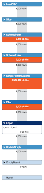I checked all of my setup multiple times, read and re-read Michael Hunger's fantastic Load CSV summary, and still was hitting problems that I should not be hitting. This is where I started looking at the query plan in more detail, and spotted the "Problem with Eager". I remembered reading one of Mark Needham's blogposts about "avoiding the Eager", and not fully understanding it as usual - but realizing that this must be what is causing the trouble. Let's drill into this a little more.

Trying to understand the "Eager Operation"

I had read about this before, but did not really understand it until Andres explained it to me again: in all normal operations, Cypher loads data lazily. See for example this page in the manual - it basically just loads as little as possible into memory when doing an operation. This laziness is usually a really good thing. But it can get you into a lot of trouble as well - as Michael explained it to me:

"Cypher tries to honor the contract that the different operations within a statement are not affecting each other. Otherwise you might up with non-deterministic behavior or endless loops. Imagine a statement like this: 

MATCH (n:Foo) WHERE n.value > 100 CREATE (m:Foo {m.value = n.value + 100}); 

If the two statements would not be isolated, then each node the CREATE generates would cause the MATCH to match again etc. an endless loop. That's why in such cases, Cypher eagerly runs all MATCH statements to exhaustion so that all the intermediate results are accumulated and kept (in memory). 

Usually with most operations that's not an issue as we mostly match only a few hundred thousand elements max. With data imports using LOAD CSV, however,  this operation will pull in ALL the rows of the CSV (which might be millions), execute all operations eagerly (which might be millions of creates/merges/matches) and also keeps the intermediate results in memory to feed the next operations in line. This also disables PERIODIC COMMIT effectively because when we get to the end of the statement execution all create operations will already have happened and the gigantic tx-state has accumulated."

So that's what's going on my load csv queries. MATCH/MERGE/CREATE caused an eager pipe to be added to the execution plan, and it effectively disables the batching of my operations "using periodic commit".  Apparently quite a few users run into this issue even with seemingly simple LOAD CSV statements. Very often you can avoid it, but sometimes you can't."

Try something different: neo4j-shell-tools

So I was wondering if there were any other ways to avoid eager, or if there would be any way for the individual cypher statement to "touch" less of the graph. That's when I thought back to a couple of years back, when we did not have an easy and convenient tool like LOAD CSV yet. In those early days of import (it's actually hard to believe that this is just a few years back - man have we made a lot of progress since that time!!!) we used completely different tools. One of those tools were basically a plugin into the neo4j-shell, called the, neo4j-shell-tools.

These tools still offer a lot of functionality that is terribly useful at times - among which a cypher-based import command, the import-cypher command. Similar to LOAD CSV, the command has a batching option, that will "execute each statement individually (per csv-line) and then batch statements on the outside so they (unintentionally, because they were written long before load csv) they circumvent the eager problem by only having one row of input per execution". Nice - so this could actually solve it! Exciting.

So then I spent about 30 mins rewriting the load csv statements as shell-tools commands. Here's an example:

//connect the Establishments to the addresses 

import-cypher -i /<path>/sourcecsv/address.csv -b 10000 -d , -q with distinct toUpper({Zipcode}) as Zipcode, toUpper({StreetNL}) as StreetNL, toUpper({HouseNumber}) as HouseNumber, {EntityNumber} as EntityNumber match (e:Establishment {EstablishmentNumber: EntityNumber}), (street:Street {name: StreetNL, zip:Zipcode})<-[:PART_OF]-(h:HouseNumber {houseNumber: HouseNumber}) create (e)-[:HAS_ADDRESS]->(h);

In this command the -i indicates the source file, -b the REAL batch size of the outside commit, -d the delimiter, and finally -q the fact that the source file is quoted. Executing this in the shell was dead easy of course, and immediately also provides nice feedback of the progress:

Just a few minutes later, everything was processed.

So this allowed us to quickly and conveniently execute all of the import statements in one convenient go. Once we had connected all the Enterprises and Establishments to the addresses, the model looks like this:

So then all that is left it to do was to connect Enterprises and Establishments to the activities:

The total import time of this entire dataset - on my Macbook Air 11 was about 3 hours - without any hickups whatsoever.

So that was a very interesting experience. Had to try lots of different approaches - but managed to get the job done.

As with the previous parts of this blog series, you can find all of the scripts etc on this gist.

In the last section of this series, we will try to summarize our lessons learnt. In any case I hope this has been a learning experience for you as well as it was for me.

Cheers

Rik

Loading the Belgian Corporate Registry into Neo4j - part 1

Every now and again, my graph-nerves get itchy. It feels like I need to get my hands dirty again, and do some playing around with the latest and greatest version of Neo4j. Now that I have a bit of a bitter team in Europe working on making Neo4j the best thing since sliced bread, that seems to become more and kore difficult to find the time to do that – but every now and again I just “get down on it” and take it for another spin.

So recently I was thinking about how Neo4j can actually help us with some of the fraud analysis and fraud detection use cases. This one has been getting a lot of attention recently, with the coming out of the Swissleaks papers from the International Consortium of Investigative Journalists (ICIJ). Our friends at Linkurio.us did some amazing work there. And we also have some other users that are doing cool stuff with Neo4j, OpenCorporates to name just one. So I wanted to do something in that “area” and started looking for a cool dataset.

The KBO dataset

I ended up downloading a dataset from the Belgian Ministry of Economics, who run the “Crossroads Database for Corporations” (“Kruispuntbank voor Ondernemingen”, in Dutch – aka as “the KBO”).  Turns out that all of the Ministry’s data on corporations is publicly available. All you need to do is register, and then you can download a ZIP file with all of the publicly registered organisations out there.

The full 200MB zip file contains a set of CSV files, holding all the data that we would possibly want for this exercise. Unzipped it’s about 1GB of data, and there’s quite a lot of it as you can see from this overview:

So you can see that this is a somewhat of a larger dataset. About 22 million CSV lines that would need to get processed – so surely that would require some thinking  … So I said “Challenge Accepted” and got going.

The KBO Model

The first thing I would need in any kind of import exercise would be a solid datamodel. So I thought a bit about what I wanted to do with the data afterwards, and I decided that it would be really interesting to look at two specific aspects in the data:

• The activitiy types of the organisations in the dataset. The dataset has a lot of data about activity categorisations – definitely something to explore.
• The addresses/locations of the organisations in the dataset. The thinking would be that I would want to understand interesting clusters of locations where lots of organisations are located.

So I created a model that could accommodate that. Here’s what I ended up with.

So as you can see, there’s quite  a few entities here, and they essentially form 3 distinct but interconnected hierarchies:

• The “orange” hierarchy has all the addresses in Belgium where corporations are located. 
• The “green” hierarchy has the different “Codes” used in the dataset, specifically the activity codes that use the NACE taxonomy. 
• The “blue” hierarchy gives us a view of links between corporations/enterprises and establishments. 

So there we had it. A sizeable dataset and a pretty much real-world model that is somewhat complicated. Now we could start thinking about the Import operations themselves.

Preparing Neo4j for the Import

Now, I have done some interesting “import” jobs before. I know that I need to take care when writing to a graph, as we are effectively doing write operations that have a lot more intricate work going on – we are writing data AND structure at the same time. So that means that we need to have some specific settings adjusted in Neo4j that would really work in our favour. Here’s a couple of things that I tweaked:

• In neo4j.properties, I adjusted the cache settings. Caching typically just introduces overhead, and when you are writing to the graph these cache really don’t help at all. So I added cache_type=weak to the configuration file.
• In neo4j-wrapper.conf, I adjusted the Java heap settings. While Neo4j is making great strides to making memory management less dependent on the Java heap, today, you should still assign a large enough heap for import operations. Now my machine only has 8GB of RAM, so I had to leave it at a low-ish 4GB on my machine. The way to force that heap size is by having the initial memory assignment be equal to the maximum memory assignment by adding two lines:

wrapper.java.initmemory=4096

wrapper.java.maxmemory=4096

to the configuration file.

That’s the preparatory work done. Now onto the actual import job.

Importing the data using Cypher’s Load CSV

The default tool for loading CSV files into Neo4j of course is Cypher’s “LOAD CSV” command. So of course that is what I used at first. I looked at the model, looked at the CSV files, and wrote the following Cypher statements to load the “green” part of the datamodel first – the code hierarchy. Here’s what I did:

create index on :CodeCategory(name); 

using periodic commit 1000load csv with headers from"file:/…/code.csv" as csvwith distinct csv.Category as Categorymerge (:CodeCategory {name: Category});

Note the “with distinct” clause in this is really just geared to make the “merge” operation easier., as we will be ensuring uniqueness before doing the merge.  The “periodic commit” allows us to batch update operations together for increased throughput. 

So then we could continue with the rest of the code.csv file. Note that I am trying to make the import operations as simple as possible on every run – rather than trying to do everything in one go. This is just to make sure that we don’t run out of memory during the operation.

create index on :Code(name); 

using periodic commitload csv with headers from"file:/…/code.csv" as csvwith distinct csv.Code as Codemerge (c:Code {name: Code}); 

using periodic commitload csv with headers from"file:/…/code.csv" as csvwith distinct csv.Category as Category, csv.Code as Codematch (cc:CodeCategory {name: Category}), (c:Code {name: Code})merge (cc)<-[:PART_OF]-(c);
create index on :CodeMeaning(description); 

using periodic commitload csv with headers from"file:/…/code.csv" as csvmerge (cm:CodeMeaning {language: csv.Language, description: csv.Description}); 

using periodic commitload csv with headers from"file:/…/code.csv" as csvmatch (cc:CodeCategory {name: csv.Category})<-[:PART_OF]-(c:Code {name: csv.Code}), (cm:CodeMeaning {language: csv.Language, description: csv.Description})merge (c)<-[:MEANS]-(cm);

As you can see from the screenshot below, this takes a while. 

If we profile the query that is taking the time, then we see that it’s probably related to the CodeMeaning query – where we add Code-meanings to the bottom of the hierarchy. We see the “evil Eager” pipe come in, where we basically know that Cypher’s natural laziness is being overridden by a transactional integrity concern. It basically needs to pull everything into memory, taking a long time to do – even on this small data-file. 

This obviously already caused me some concerns. But I continued to add the enterprises and establishments to the database in pretty much the same manner:

//load the enterprises
create constraint on (e:Enterprise)assert e.EnterpriseNumber is unique;
using periodic commit 5000load csv with headers from"file:/…/enterprise.csv" as csvcreate (e:Enterprise {EnterpriseNumber: csv.EnterpriseNumber, Status: csv.Status, JuridicalSituation: csv.JuridicalSituation, TypeOfEnterprise: csv.TypeOfEnterprise, JuridicalForm: csv.JuridicalForm, StartDate: toInt(substring(csv.StartDate,0,2))+toInt(substring(csv.StartDate,3,2))*100 + toInt(substring(csv.StartDate,6,4))*10000});

Note that I used a nice trick (described in this blogpost) to convert the date information in the csv file to a number. 

//load the establishments
create constraint on (eb:Establishment)assert eb.EstablishmentNumber is unique; 

using periodic commitload csv with headers from"file:/…/establishment.csv" as csvcreate (es:Establishment {EstablishmentNumber: csv.EstablishmentNumber, StartDate: toInt(substring(csv.StartDate,0,2))+toInt(substring(csv.StartDate,3,2))*100+toInt(substring(csv.StartDate,6,4))*10000}); 

using periodic commitload csv with headers from"file:/…/establishment.csv" as csvmatch (e:Enterprise {EnterpriseNumber: csv.EnterpriseNumber}), (es:Establishment {EstablishmentNumber: csv.EstablishmentNumber})create (es)-[:PART_OF]->(e);

Interestingly, all of this is really fast. 

Especially if you look at what was happening above with the Code-meanings. The reson for this is of course the fact that we are doing a lot simpler operations here while adding the data. The entire execution time on my little laptop was  7 minutes and 10 seconds to add 3180356 nodes and 1602575 relationshipts. Not bad at all.

At this point the model looks like this:

Then we start working with the address data, and start adding this to the database. It works very well for the Cities and Zipcodes:

create constraint on (c:City)
assert c.name is unique; 

create constraint on (z:Zip)
assert z.name is unique; 

create index on :Street(name); 

//adding the cities
using periodic commit 100000
load csv with headers from
"file:/…/address.csv" as csv
with distinct toUpper(csv.MunicipalityNL) as MunicipalityNL
merge (city:City {name: MunicipalityNL}); 

//adding the zip-codes
using periodic commit 100000
load csv with headers from
"file:/…/address.csv" as csv
with distinct toUpper(csv.Zipcode) as Zipcode
merge (zip:Zip {name: Zipcode}); 

// connect the zips to the cities
using periodic commit 100000
load csv with headers from
"file:/…/address.csv" as csv
with distinct toUpper(csv.Zipcode) as Zipcode, toUpper(csv.MunicipalityNL) as MunicipalityNL
match (city:City {name: MunicipalityNL}), (zip:Zip {name: Zipcode})
create unique (city)-[:HAS_ZIP_CODE]->(zip);

Once we have this, we then wanted to add the streets to the Zip - not to the city, because we can have duplicate streetnames in different cities. And this is a problem:

It takes a very long time. The plan looks like this:

And unfortunately, it gets worse for adding the  HouseNumbers to every street. It still works – but it’s painfully slow.

I tried of different things, called the help of a friend, and finally got it to work by replacing “Merge”by “Create Unique”. That operation does a lot less checking on the total pattern that you are adding, and can therefore be more efficient. So oof. That worked. 

Unfortunately we aren’t done yet. We still need to connect the Enterprises and Establishments to their addresses. And that’s where the proverbial sh*t hit the air rotating device – and when things stopped working. So we needed to address that, and that;s why there will be a part 2 to this blogpost very soon explaining what happened. 

All of the material mentioned on this blog series is on github if you want to take a look at it.

Hope you already found this useful. As always, comments are very welcome.

Cheers

Rik