Cycling Tweets Part 4: Ranking the Nodes

In the previous couple of blogposts in this series (here's part 1, part 2 and part 3 for you), I have explained how I got into the Cycling Twitterverse, how I imported data from a mix of sources (CQ Ranking, TwitterExport, and a Python script talking to the Twitter API), and thereby constructed a really interesting graph around Cycling.

There's so many more things to do with this dataset. But in this post, I want to explore something that I have been wanting to experiment with for a while: The GraphAware Framework. Michal and his team have been doing some real cool stuff with us in the past couple of years, not in the least the creation of a couple of very nice add-ons/plugins to the Neo4j server.

One of these modules is the "NodeRank" module. This implements the famous "PageRank" algorithm that made Google what it is today.

It does this in a very smart way - and also very unintrusively, utilising only excess capacity on your Neo4j server. It's really easy to use. All you need to do is

• drop the runtimes in the Neo4j ./plugins directory
• activate the runtimes in the Neo4j.properties file that you find in your Neo4j ./conf directory. 

Here's what I added to my server (also available on github):

//Add this to the <your neo4j directory>/conf/neo4j.properties after adding
//graphaware-noderank-2.2.1.30.2.jar and
//graphaware-server-enterprise-all-2.2.1.30.jar
//to <your neo4j directory>/plugins directory
 
com.graphaware.runtime.enabled=true
 #NR becomes the module ID:
com.graphaware.module.NR.1=com.graphaware.module.noderank.NodeRankModuleBootstrapper
 
#optional number of top ranked nodes to remember, the default is 10
com.graphaware.module.NR.maxTopRankNodes=50
 
#optional damping factor, which is a number p such that a random node will be selected at any step of the algorithm
#with the probability 1-p (as opposed to following a random relationship). The default is 0.85
com.graphaware.module.NR.dampingFactor=0.85
 
#optional key of the property that gets written to the ranked nodes, default is "nodeRank"
com.graphaware.module.NR.propertyKey=nodeRank
 
#optionally specify nodes to rank using an expression-based node inclusion policy, default is all business (i.e. non-framework-internal) nodes
com.graphaware.module.NR.node=hasLabel('Handle')
 
#optionally specify relationships to follow using an expression-based relationship inclusion policy, default is all business (i.e. non-framework-internal) relationships
com.graphaware.module.NR.relationship=isType('FOLLOWS') #NR becomes the module ID:
com.graphaware.module.TR.2=com.graphaware.module.noderank.NodeRankModuleBootstrapper
 
#optional number of top ranked nodes to remember, the default is 10
com.graphaware.module.TR.maxTopRankNodes=50
 
#optional damping factor, which is a number p such that a random node will be selected at any step of the algorithm
#with the probability 1-p (as opposed to following a random relationship). The default is 0.85
com.graphaware.module.TR.dampingFactor=0.85
 
#optional key of the property that gets written to the ranked nodes, default is "nodeRank"
com.graphaware.module.TR.propertyKey=topicRank
 
#optionally specify nodes to rank using an expression-based node inclusion policy, default is all business (i.e. non-framework-internal) nodes
com.graphaware.module.TR.node=hasLabel('Hashtag')
 
#optionally specify relationships to follow using an expression-based relationship inclusion policy, default is all business (i.e. non-framework-internal) relationships
com.graphaware.module.TR.relationship=isType('MENTIONED_IN')

As you can see from the above, I have two instances of the NodeRank module active. 

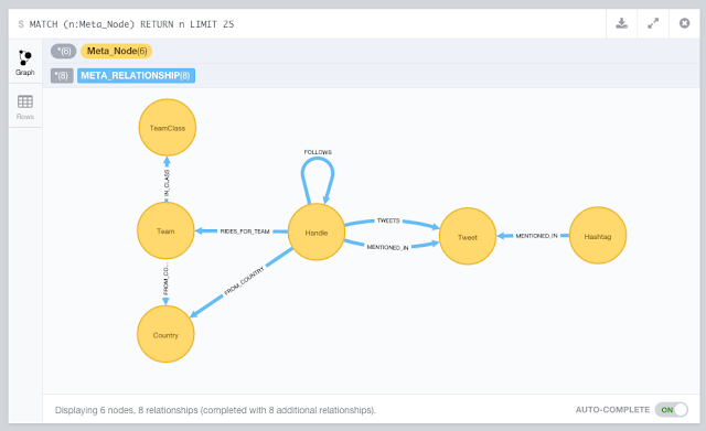
1. The first attempts to get a feel for the importance of "Nodes" (in this case, the nodes with label "Handle") by calculating the nodeRank along the "FOLLOWS" relationships. After just half an hour of "ranking" we get a pretty good feel:
   
   This seems to be confirming - in my humble opinion - some of the more successful riders in April, for sure. But also confirms that the "big names" (Contador, Froome, Cancellara) are attracting their share of Twitter activity no matter what.
2. The second does the same for the "Topics" (in this case, the nodes with the label "Hashtag") along the the "MENTIONED_IN" relationships.
   
   The classic races are clearly "top of mind" in the Twitterverse! But upon investigation I have also found that there are a lot of confusing #hashtags out there that make it difficult to understand the really important ones. Would love to investigate a bit more there.

Like I said before, the GraphAware framework is really interesting. It gives you the opportunity to make stuff that you could also do in Cypher more easily, faster, and more consistently. I really liked my experience with it.

Hope this was useful for you - as always feedback is very very welcome.

Cheers

Rik

Cycling Tweets Part 3: Adding "Friends" to the CyclingGraph

In this 3rd part of this blogpost series about Cycling (you can find part 1 and part 2 in earlier posts) we are going to take the existing Neo4j dataset a bit further. We currently have the CQ Ranking metadata in there, the tweets that we exported all connected up to the riders' handles, and then we analysed the tweets for @handle and #hashtag mentions. We got this:

Now my original goal included having a social graph in there too: the "friends" relationships for different twitterers could be interesting too. Friends are essentially two-way follow-relationships - where two handles follow each other, thereby indicating some kind of closer relationship. It's neatly explained over here. So how to get to those?

Well, I did some research, and while there are multiple options, my conclusion was that really you would need to have a script that would talk to the twitter API. And since we also know that IANAP (I AM Not A Programmer), I would probably need a little help from my friends.

Friends to the rescue: my first python script

Turns out that my friend and colleague Mark Needham had already done some work on a very similar topic: he had developed a set of Python scripts that used the Tweepy library for reading from the Twitter API, and Nigel Small's Py2Neo for writing to Neo4j.  So I started looking at these and found them surprisingly easy to follow.

So I took a dive at the deep end, and started to customize Mark's scripts. I actually spent some time going through a great python course at Codecademy, but really my tweaks to Mark's script could have been done without that too. His original script had two interesting arguments that I decided to morph:

• --download-all-user-profiles
  I tweaked this one to "download all user friends" from the users.csv file. The new command is below.
• --import-profiles-into-neo4jI tweaked this one to "import all friends into neo4j" from the .json files in the ./friends directory. The new command is also below.

In order to use this, you do need to put in placeI have put my final script over here for you to take a look. In order to use it, you have to register an App at Twitter, and generate credentials for the script to work with:

That way, our python script can read stuff directly from the Twitter API. Don't forget to "source" the credentials, as explained on Mark's readme.

2 new command-line arguments

Mark's script basically uses a number of different command-line arguments to do stuff. I decided to add two arguments. The first argument I added was

python twitter.py --download-all-user-friends 

This one talks to the Twitter API, and downloads the friends of all the users that it found in the users.csv file.  I generated that file based on the CQ ranking spreadsheet that I had created earlier.

As you can see, it pauses when the "rate limit" is reached - this is standard Tweepy functionality. The output is a ./friends directory full of .json files. Here's an example of such a file (tomboonen1.json)

In these .json files there is a "friends" field. Using the second part of the twitter.py script, we can then import these friends to our existing Neo4j CyclingTweets database using the following Cypher statement (note that the {variables} in green are Python variables, the rest is pure Cypher):

"""
MATCH (p:Handle {name: '@'+lower({screenName})})
SET p.twitterId = {twitterId}
WITH p
WHERE p is not null
UNWIND {friends} as friendId
MATCH (friend:Handle {twitterId: friendId})
MERGE (p)-[:FOLLOWS]->(friend)
"""

So essentially this finds the screenName (aka the "handle"), adds the twitterId to the screenName, and then adds the "FOLLOWS" relationships between that handle and the friends of that handle. Pretty sweet.

So let's run the script, but this time with a different command line argument, and with a running Neo4j server in the background that the script could talk to:

python twitter.py --import-friends-into-neo4j

After a couple of minutes (if that), this is done, and we have a shiny new graph that includes the FOLLOWS relationships:

This is pretty much what I set out to create in the first place, but thanks to the combination of the import (part 2) and this Python script - I have actually got a whole lot more info in my dataset. Some very cool stuff.

Hope you liked this 3rd part of this blogpost series. There's so much more we could do so - so look out for part 4 soon!

Cheers

Rik

Cycling Tweets Part 2: Importing into Neo4j

So after completing the first part of this blogpost series, I had put together a bit of infrastructure to easily import data into Neo4j. All the stuff was now in CSV files and ready to go:
So I got out my shiny new Neo4j 2.2.1, and started using Load CSV for getting the data in there. Essentially there were three steps:

• Importing the metadata about the riders and their twitter handles: importing the metadata
• Importing the actual tweets
• Processing the actual tweets

So let's go through this one by one. We will be using the following model to do so:

 

1. Importing the Cycling metadata into Neo4j

I wrote a couple of Cypher statements to import the data from CQ ranking:

//add some metadata
//country info
load csv with headers from 
"https://docs.google.com/a/neotechnology.com/spreadsheets/d/1lLD2I_czto1iA1OjCMAZZxnYLAVsngBgjT5c0xuvpJ0/export?format=csv&id=1lLD2I_czto1iA1OjCMAZZxnYLAVsngBgjT5c0xuvpJ0&gid=1390098748" as csv
create (c:Country {code: csv.Country, name: csv.FullCountry, cq: toint(csv.CQ), rank: toint(csv.Rank), prevrank: toint(csv.Prev)});
 
//team info
load csv with headers from"https://docs.google.com/a/neotechnology.com/spreadsheets/d/1lLD2I_czto1iA1OjCMAZZxnYLAVsngBgjT5c0xuvpJ0/export?format=csv&id=1lLD2I_czto1iA1OjCMAZZxnYLAVsngBgjT5c0xuvpJ0&gid=1244447866" as csv
merge (tc:TeamClass {name: csv.Class})
with csv, tc
match (c:Country {code: csv.Country})
merge (tc)<-[:IN_CLASS]-(t:Team {code: trim(csv.Code), name: trim(csv.Name), cq: toint(csv.CQ), rank: toint(csv.Rank), prevrank: toint(csv.Prev)})-[:FROM_COUNTRY]->(c);
 
//twitter handle info
using periodic commit 500load csv with headers from 
"https://docs.google.com/a/neotechnology.com/spreadsheets/d/1lLD2I_czto1iA1OjCMAZZxnYLAVsngBgjT5c0xuvpJ0/export?format=csv&id=1lLD2I_czto1iA1OjCMAZZxnYLAVsngBgjT5c0xuvpJ0&gid=0" as csv
match (c:Country {code: trim(csv.Country)})
merge (h:Handle {name: trim(csv.Handle), realname: trim(csv.Name)})-[:FROM_COUNTRY]->(c);
 
//rider info
load csv with headers from 
"https://docs.google.com/a/neotechnology.com/spreadsheets/d/1lLD2I_czto1iA1OjCMAZZxnYLAVsngBgjT5c0xuvpJ0/export?format=csv&id=1lLD2I_czto1iA1OjCMAZZxnYLAVsngBgjT5c0xuvpJ0&gid=1885142986" as csv
match (h:Handle {realname: trim(csv.Name)}), (t:Team {code: trim(csv.Team)})
set h.Age=toint(csv.Age)
set h.CQ=toint(csv.CQ)
set h.UCIcode=csv.UCIcodeset h.rank=toint(csv.Rank)
set h.prevrank=toint(csv.Prev)
create (h)-[:RIDES_FOR_TEAM]->(t);
 
//add the index on Handle
create index on :Handle(name);
create index on :Hashtag(name);
create index on :Tweet(text);
create index on :Handle(nodeRank);
create constraint on (h:Handle) assert h.twitterId is unique;

As you can see, I also added some indexes. The entire script is also on Github.

The graph surrounding Tom Boonen now looked like this:

Once I had this, I could start adding the actually twitter info. That's next.

2. Importing the tweet data into Neo4j

As we saw previously, I had one CSV file for every day now. So how to iterate through this? Well, I did it manually, and create a version of this query for every day between April 1st and 30th.

//get the handles from the csv file
//this should not do anything - as the handles have already been loaded above
using periodic commit 500load csv with headers from "file:<yourpath>/20150401.csv" as csv
with csv
where csv.Username<>[]
merge (h:Handle {name: '@'+lower(csv.Username)});
  //connect the tweets to the handles
using periodic commit 500load csv with headers from "file:<your path>/20150401.csv" as csv
with csv
where csv.Username<>[]
merge (h:Handle {name: '@'+lower(csv.Username)})
merge (t:Tweet {text: lower(csv.Tweet), id: toint(csv.TweetID), time: csv.TweetTime, isretweet: toint(csv.IsReTweet), favorite: toint(csv.Favorite), retweet: toint(csv.ReTweet), url: csv.`Twitter URL`})<-[:TWEETS]-(h);

This file is also on Github, of course. I ran this query 30 times, replacing 20150401 with 20150402 etc etc... The result looked like this:

But obviously this is incomplete: we only have the tweets issued by specific riders now - and we would really like to know who and what they mentioned - in other words extract the handles and hashtags from the tweets. Let\s do that!

3. Processing the tweets: Extract the handles and the hashtags

I created two queries to do this - they are also on Github:

//extract handles from tweet text and connect tweets to handles
match (t:Tweet)
WITH t,split(t.text," ") as words
UNWIND words as handles
with t,handles
where left(handles,1)="@"with t, handles
merge (h:Handle {name: lower(handles)})
merge (h)-[:MENTIONED_IN]->(t);
 
//extract hashtags from tweet text and connect tweets to hashtags
match (t:Tweet)
WITH t,split(t.text," ") as words
UNWIND words as hashtags
with t,hashtags
where left(hashtags,1)="#"with t, hashtags
merge (h:Hashtag {name: upper(hashtags)})
merge (h)-[:MENTIONED_IN]->(t);

And that's when we start to see the twitter network unfold: multiple riders tweeting and mentioning eachother:

That's about it for this part 2. In the next section we will go into how we can enrich this dataset with more data about the connectedness between riders. Who is following who?

I hope you have liked this series so far. As always, feedback very welcome.

Cheers

Rik

Cycling Tweets Part 1: Who's who on Twitter

I have been a Cycling fan for a long time. Got into it at University a long time ago through some crazy friends that were already into it. And I have been on the bike ever since. Whether it's just for some grocery shopping and/or bar hopping in Antwerp, or for a longer holiday trip - or just for watching the pro riders in  CycloCross or Road racing - I am game for all of it. I even got my boys really excited about - watching legendary races like the Tour of Flanders or Paris-Roubaix together religiously.

So last March, I was thinking of yet another crazy Neo4j-experiment to do, and I thought about doing that on some cycling topics. After all, April is a "Holy Month" for cycling enthousiasts - many of the legendary "classic races" are happening during that month. So that's what I did. I will be detailing this over the next couple of blogposts - but suffice to say that I got into a bit of a project here, a journey that I gladly want to share with you.

So here it goes. This is part 1 of (what I think will be) 5 blogposts around Neo4j, graph databases, Twitter and Cycling. Hoping you will enjoy it.

Starting with the riders

The obvious idea I had was to try and do some work with some social networking data for the top riders in the pro cycling peloton. I follow some of these guys myself on my Twitter feed, but how would I be able to get to all the interesting ones like Tom Boonen, Fabian Cancellara, and others. I googled around a bit and found this site: CQ Ranking. In their own words: they are a ranking of Pro cycling riders that try to rank riders based on the past 12 performance - a bit like the UCI ranking of cyclists. And they provide some really cool data: here's an example of a sheet that you can download from their website.

One of the most interesting data elements that I found on the CQ website was the list of Twittering riders. This was almost exactly what I was looking for for my experiment, a long list of all the riders, their teams, their countries... and their twitter handles. Obviously there were going to be some mistakes/problems in this list, but still - it looked pretty sweet. So there I went, downloading everything and putting it all into a google spreadsheet for some data cleanup so that I could prepare it for an upload into Neo4j.

The only real thing that I had to do was to match the CQ ranking sheet with the with twittering riders. That was easy enough once I had both data sets different tabs of the google sheet: a simple VLOOKUP was all it took:

And then we got this sheet:

Interesting. Now I have a list of very interesting twitter accounts - what to do with them. This is when the first part of my experiment really started to materialise, and when I decided that I would love to know what all these interesting online characters would be up to in a Holy (!) month like this one. I would love to know what they were tweeting about, who they were mentioning, how they would be grouped together etc... So I needed to get to that data... 

Getting to the Twitter data

This turned out to be a bit more difficult than I thought it would be. Sure, Twitter gives you this API access to read from their vast datasets, but frankly, for a newbie like me these "rate limiting" rules are pretty confusing and intransparant. And plus - I don't really know how to code :) - so that really limited my options. So I tried a few things and then decided that the easiest way to get to all of these "April tweets" would be to create a new twitter account  (CycleF0ll0w) and then follow all of the accounts that I wanted to follow (from the spreadsheet). So that's what I did: a ghost twitter ID appeared: all it does is follow people - so that I have access to the timeline that contains the information I want.

In order to easily create the list of people that "I" followed, I used a tool called Tweepi: it allows for bulk creation of "follow" links really easily. I decided to go with the top 500 (as per their CQ ranking) riders - that should be more than interesting enough.

Exporting and Cleaning the timeline

So now I have a timeline. How do I get that to be extracted so that I can work with it and get it ready to be imported into Neo4j? Again, I investigated multiple options, but ended up going for a paid service: Exporttweet. On a daily basis, this service automatically created an Excel spreadsheet containing all the tweets appearing on my CycleF0ll0w timeline.

The output was really simple: an Excel file a day, keeps the doctor away!

Now all there was left to do was to clean these sheets up a bit. I used my tried and tested Open Refine install to do that:

It was mostly taking out special characters, renaming column names, and removing duplicates, and I ended up with a very simple set of Replay Refine operations based on the saved json file:

That was it. Now I had everything ready to get started:

• a google doc with a bunch of metadata about riders (names, teams, rankings, twitter handles)
• a timeline with all the tweets of these riders, and a way to export that into daily XLS files
• an OpenRefine process to create CSV files out of these tweets on a daily basis. 

In the next blog post I will go and get started with this - and start having some fun with the data.

Hope you enjoyed this so far - already looking forward to part 2. As always, feedback welcome.

Cheers

Rik

Importing the SNAP Beeradvocate dataset into Neo4j - part 1

As you may or may not know, I am a big fan of Beer. And I am a big fan of Neo4j. I did a talk about this at GraphConnect two years ago ...

- and I have been doing that demo a lot with lots of users, customers and meetups. Up to the point where I was really working up a reputation as a "Beer Guy". Not sure if that is good or bad...

So some time ago I learned about the SNAP: Stanford Network Analysis Project, who mention an example dataset that is really interesting: 1.5 million Beer-reviews from Beeradvocate between January 1998 and November 2011. Here are some stats:
And then at the bottom of the page it says:

Disappointment!!! But then one simple Google search led me to this blob and a 445 Mbyte download later, we were in business. Unzip the thing, and we have a 1.5Gbyte text file to play with.

Importing the data? Not quite, yet!

Once I had downloaded the data, I found that there were two big "bears" on the road. Two problems that I would have to solve.

• Problem 1: the size of the data. I would not really call this file huge, but on my little laptop (I "only" have 8gbyte of RAM on my machine) it can get kind of tricky to work with biggish files like that... Based on experience - I just know I will get into trouble, and will need to work around that.
• Problem 2: the structure of the data. Here's a look at the file:

This definitely does not look very Neo4j-import friendly. I need to do some transformations there to make the thing easy to import.

So how did I go about solving this? Read on.

Solution 1: splitting the text file

The first thing I set out to do was to split the text file into different parts, so that it would be easier to handle and transform along the way. I looked around for a while, and then found the split bash command - by far the simplest, most performant and straightforward option.  Played around with different options (different sizes for the splits - I first had 6 files, then 3, and ended up choosing to split into 15 100 Mbyte files), and eventualy used this simple command:

split -b 100m beeradvocate.txt

This was the result

Nice - 15 perfectly manageable files! Once done that, needed to assure that the split was not completely arbitrary, and that "whole records" were included in every file. Easy peasy with some simple copying and pasting from the end of each file to the beginning of the next file - done in less than 5 minutes! Job done!

Solution 2: transforming the .txt files

Then I needed to get these manageable files into a .csv format that I could import into Neo4j. This was more complicated. I needed to go 

• from a structure that had records in blocks of 14 lines, with a property field on every line
• to a .csv file that had a row per record, and fields in comma-separated columns

That's quite a transformation, for which I would need some tooling. I decided on trying OpenRefine. I had heard about this tool a couple of years ago already, but never made any serious use of it. Now I thought it would come in handy, as I would have to go through every step of the transformation 15 times - once for every .txt file that we generated above.

So I fired it up, and created the first of 15 "projects" in Refine. This is what it looked like before the transformation :

After one parsing operation using the "line-based text file" transformation, I already got a preview that looked like this:

Already looks kind of right - at least I already have a row per record now.

Now I would need to do some manipulations before the text file became usable. Google refine has this really wonderful transformation tool that allows you to create manipulation steps that you can execute and process step after step. The main steps were:

• extracting the "field name" from every cell, and just leave the data in there. Every cell currently was structured as "<<field name>>: <<field value>>", and I would want every cell to just contain the "<<field value>>".
• renaming the columns so that my .csv file would have nice workable headers. This is not mandatory - but I found that easier.

When you do this manually, it can be a bit cumbersome and repetitive - so you definitely don't want to do this 15 times. That's where Refine is so nice: you can extract a .json file that specifies all the operations, and then apply these operations to forthcoming "projects" afterwards time and time again.

So you do it once, and then you can extract that .json so that you can use it later on the other 14 files - which is exactly what I wanted.

That .json file is also on github.

The result was exactly what we wanted: a comma-separated file that would be ready for import into Neo4j.

Download the file and we are done with the import preparations for this file. Of course you would need to do this 15 time, but thanks to the .json file with the operations steps, that was really easy.

You can find the sample files (of both the .txt file, the Refine operations .json and the resulting .csv file) are on github.

That was it for part 1. We now have everything ready to do an import. In part 2 we will do the actual import into Neo4j and start playing around with it.

Hope you enjoyed this.

Cheers

Rik

PS: Here are the links to

• Part 2
• Part 3