Same .CSV files, different neo4j database!

As you probably know, Neo Technology is getting closer and closer to releasing the major new release of the neo4j database: version 2.0. Going from 1.9.x to 2.0 is a bigger jump than you may expect. It's not just a 0.1 difference ;-) ... 2.0M06 is jam-packed with new features, among which the fantastic new extension to the property graph data model: node labels.

Labels are simply fantastic in my opinion. You can read up on the advantages that they bring, now and into the future, over here. But what does it mean to some of my previously generated neo4j databases? Well - turns out it's quite a thing. Not that the actual upgrade of the datastore is difficult (it's as simple as uncommenting the "allow_store_upgrade=true" line in the neo4j.properties file), but how could I actually start taking advantage of the labels feature, in my datamodel, in my queries, in the fantastic new neo4j browser? Let's find out.

Revisiting my Last.fm model

In my previous blog posts, I had imported a last.fm scrobbling dataset using different methods. The model looked something like this:

In all of the nodes of that model, I had included at minimum two properties: a "name" and a "type". So guess what: it makes total sense to convert these "type" properties into labels, ending up with 6 different subgraphs based on the labels: listeners, scrobbles, tracks, artists, albums and dates. Nice. I will be able to use the new, improved indexing that neo4j 2.0 features based on these labels, of course.

Re-importing the data from the same .csv files

So then I need to recreate the database reflecting this change. My source files (see the previous blogpost: just download from here) are of course the same - all I need was a slightly modified import process. My dear friend Michael Hunger has already prepared a 2.0 version of the neo4j-shell-tools - and they just work like a charm. 

Here are the import statements for the nodes:

import-cypher -d ; -i ./IMPORT/INPUT/nodespart1.csv -o ./IMPORT/OUTPUT/1out.csv create (n:#{type} {name:{name}}) return n.name as name

import-cypher -d ; -i ./IMPORT/INPUT/nodespart2.csv -o ./IMPORT/OUTPUT/2out.csv create (n:#{type} {title:{title}, name:{name}}) return n.name as name

As you can suspect, the n:#{type} piece is the interesting part. This is where we use the "type" data-element from the csv files for the labels, not for the old "type-property". The reason why the # is there is because Michael had to do some wizardry to allow for parametrized labels - which is normally not supported in Cypher.

Adding indexes based on Labels 

Before we now go and import the relationships, we have to add the indexes on these newly created nodes and labels. We do that as follows in the neo4j-shell:

CREATE index on :date(name);  

CREATE index on :album(name);  

CREATE index on :scrobble(name);  

CREATE index on :listener(name);  

CREATE index on :artist(name);  

CREATE index on :track(name); 

This takes a second or two. but once complete, we can see that the indexes are ready to be used by typing the schema command:

And then we can proceed to import the relationships, again with the same .csv files.

No longer starting with a start

Importing the relationships is also done with neo4j-shell-tools, but slightly different from last time: the parametrized cypher queries no longer "start with a START", they now start with a "MATCH". This is because, now that indexing has become an integral part of neo4j, you can really work with Cypher in an even more declarative fashion than before. You don't have to imperatively tell the database where to start - it will figure it out for you based on the pattern that you specify.

Here are the new import statements:

import-cypher -d ; -i ./IMPORT/INPUT/APPEARS_ON.csv -o ./IMPORT/OUTPUT/3out.csv MATCH (track:track), (album:album) where track.name={mbid1} and album.name={mbid2} create unique track-[:APPEARS_ON]->album return track.name, album.name

import-cypher -d ; -i ./IMPORT/INPUT/CREATES.csv -o ./IMPORT/OUTPUT/4out.csv MATCH (album:album), (artist:artist) where artist.name={mbid1} and album.name={mbid2} create unique artist-[:CREATES]->album return album.name, artist.name

import-cypher -d ; -i ./IMPORT/INPUT/FEATURES.csv -o ./IMPORT/OUTPUT/5out.csv MATCH (scrobble:scrobble), (track:track) where scrobble.name={scrobble} and track.name={mbid} create unique scrobble-[:FEATURES]->track return scrobble.name, track.name

import-cypher -d ; -i ./IMPORT/INPUT/LOGS.csv -o ./IMPORT/OUTPUT/6out.csv MATCH (listener:listener), (scrobble:scrobble) where listener.name={user} and scrobble.name={song} create listener-[:LOGS]->scrobble return listener.name, scrobble.name

import-cypher -d ; -i ./IMPORT/INPUT/ON_DATE.csv -o ./IMPORT/OUTPUT/7out.csv MATCH (date:date), (scrobble:scrobble) where scrobble.name={song} and date.name={date} create scrobble-[:ON_DATE]->date return scrobble.name, date.name

import-cypher -d ; -i ./IMPORT/INPUT/PERFORMS.csv -o ./IMPORT/OUTPUT/8out.csv MATCH (artist:artist), (track:track) where artist.name={mbid1} and track.name={mbid2} create unique artist-[:PERFORMS]->track return artist.name, track.name

import-cypher -d ; -i ./IMPORT/INPUT/PRECEDES.csv -o ./IMPORT/OUTPUT/9out.csv MATCH (date1:date), (date2:date) where date1.name={date1} and date2.name={date2} create date1-[:PRECEDES]->date2 return date1.name, date2.name

You can download the entire set of statements from over here.

So there we have it: a newly imported, nicely labeled neo4j-2.0 dataset. So let's fire up the browser and see what the result looks like?

Very nice! Now I can start playing around to my hearts' content with the new browser and have even more fun. How is that even possible?

Hope this was useful. Until next time.

GraphConnect Video treasures!

You should really be taking a look at all the wonderful GraphConnect San Francisco videos on watch.neo4j.org - they are simply awesome. So much detail wonderful information in these talks - it's just such a pleasure to watch. Oh, and in case you're interested, here's my little beertalk:
Graphs and Beer - Rik Van Bruggen @ GraphConnect SF 2013 from Neo Technology on Vimeo.

Hope you enjoy!

Importing my Last.fm dataset - the neo4j way

Some time ago, I blogged about how you could create an interesting graph dataset in neo4j using the data from Last.fm. At the time, I used Talend as an ETL tool, to do the import into neo4j – as the dataset was quite large and the spreadsheet method would probably not cut it anymore. It worked great – the only downside (for this particular use case) was that ... I had to learn Talend. And not that that is terribly difficult – especially not if you are an experienced ETL professional, which I am clearly NOT – but there was definitely a learning curve involved. So: there continued to be a latent desire to do this import into neo4j natively – without separate tooling. And now, I think we have that, thanks to the ever-amazing Michael Hunger.

Enter neo4j-shell-tools

Michael created a collection of utilities that basically plug into the neo4j-shell, and extend its functionalities with things like... data import functionalities. There are different options, and you should definitely read up on the different capabilities, but for my specific Last.fm use case, what was important was that it can easily import the csv files that I had created at the time for the import using talend.

You can read up on the details of the shell-tools in the readme (in contains very simple installation instructions that you would need to go through beforehand – essentially installing the .jar file in neo4j's lib directory). Once you have done that and you shutdown/restart the neo4j server, you are good to go.

Creating the database from scratch.

As you will see below, the steps are quite simple:

Step 1: start with an empty neo4j database

What's important here is that the neo4j-shell-tools work on a **running** neo4j database. You do not need to introduce downtime, and you do not use the so-called “batchimporter” method – instead you are doing a full blow, transactional, live update on the graph, using this toolset.

Step 2: prepare the .csv files

I had already prepared these files for the previous blogpost – so that was easy. The only difference that I had to make was that I

• had to make sure that the delimiter that I was using was right. The neo4j-shell-tool allows you to specify the type of delimiter, and getting that wrong will obviously lead to faulty imports
• had to add a “header” row at the top of the text files. The neo4j-shell-tool will assume that the first line of the .csv files defines the structure of the rest of the file. Which also then means, that I needed multiple files as both the nodes and relationships that I wanted to add have a different structure/type.

So I ended up with 2 .csv files to add nodes to the graph, and 7 .csv files to add the relationships between the nodes. You can download everything here.

Step 3: prepare the import commands

The node import commands look like this

import-cypher -d ; -i nodespart1.csv -o 1out.csv create (n{name:{name}, type:{type}}) return n.name as name

import-cypher -d ; -i nodespart2.csv -o 2out.csv create (n{title:{title}, name:{name}, type:{type}}) return n.name as name

The structure of these commands is fairly simple:

• import-cypher: calls the shell tool that we want to use
• -d defines the delimiter of the file that we are importing. In these case a “;”.
• -i defines the input file. On OSX, not adding a path will just look for the file in the root of your neo4j installation directory. In many cases you will want to have an absolute, or relative path from there.
• -o defines an option output file where the result of the import commands will be written. This is intended for logging purposes.
• And then finally, with the highlighted “create...” section, we basically define the Cypher query that will do the import transaction – using the parameters from the csv file (between { }) as input.

Note that the neo4j-shell-tools provide some separate functionalities for dealing with large input files and for tuning the transaction throttling (how many updates in one transaction), but that for this purpose we really did not need to do that.

Then for the relationship import commands, we have a very similar structure:

import-cypher -d ; -i APPEARS_ON.csv -o 3out.csv start n1=node:node_auto_index(name={mbid1}), n2=node:node_auto_index(name={mbid2}) create unique n1-[:APPEARS_ON]->n2 return n1.name, n2.name

import-cypher -d ; -i CREATES.csv -o 4out.csv start n1=node:node_auto_index(name={mbid1}), n2=node:node_auto_index(name={mbid2}) create unique n1-[:CREATES]->n2 return n1.name, n2.name

import-cypher -d ; -i FEATURES.csv -o 5out.csv start n1=node:node_auto_index(name={scrobble}), n2=node:node_auto_index(name={mbid}) create unique n1-[:FEATURES]->n2 return n1.name, n2.name

import-cypher -d ; -i LOGS.csv -o 6out.csv start n1=node:node_auto_index(name={user}), n2=node:node_auto_index(name={song}) create n1-[:LOGS]->n2 return n1.name, n2.name

import-cypher -d ; -i ON_DATE.csv -o 7out.csv start n1=node:node_auto_index(name={scrobble}), n2=node:node_auto_index(name={date}) create n1-[:ON_DATE]->n2 return n1.name, n2.name

import-cypher -d ; -i PERFORMS.csv -o 8out.csv start n1=node:node_auto_index(name={mbid1}), n2=node:node_auto_index(name={mbid2}) create unique n1-[:PERFORMS]->n2 return n1.name, n2.name

import-cypher -d ; -i PRECEDES.csv -o 9out.csv start n1=node:node_auto_index(name={date1}), n2=node:node_auto_index(name={date2}) create n1-[:PRECEDES]->n2 return n1.name, n2.name

Note that, because of the domain model that we have from the last.fm dataset, some relationships have to be unique and others don't – hence the difference in the Cypher queries.

Step 4: executing the commands

Then all we need to do is to put the files on the right locations, make sure that autoindexing is correctly defined, and then copy/paste the commands into the neo4j-shell.

On my MacBook Pro, the entire import took about 35 seconds, and I ended up with the database that I had previously created with the Talend toolset:

And then the same graphic/query exploration can begin. You can take the graphical tools for a spin, or alternatively create your own cypher queries and get going.

Conclusion

Overall, I found this new process to be extremely intuitive and straightforward – even simpler then what I had experienced using the Talend toolset. I have put the zip-file and the corresponding input statements over here – so feel to download and experiment yourself. Just make sure that you put the .csv files in the neo4j “home directory”, or adjust the paths as you want (both relative and absolute paths seemed to work on my machine).

Hope this was useful. Until the next time!

Rik

Connecting NeoOffice to Neo4j

Lots of people have blogged about using the jdbc driver for neo4j. This was a project that was initially created by Rickard Oberg, and has been released quite some time ago for neo4j 1.9 and 2.0. Take a look at the neo4j.org jdbc page for many different examples and desscriptions.

In this blogpost, I will be focussing on one of the integrations that could be very useful for non-technical, end-user computing style people like myself. I have blogged before about how you can use a spreadsheet to import data into neo4j, but now, what I would like to demonstrate here is how easy it is to generate a spreadsheet with data that is coming straight from a neo4j cypher query. Let’s say that I have a complex query, one with multiple “joins” and that I am using neo4j to get neo4j to get some decent performance on these queries.

So what do I need:

• a running neo4j database. I will use my beergraph as a dataset and run some of these queries as examples.
• the jdbc driver. Download the binaries and install them. Dead simple. Detailed instructions are on the github page.
• NeoOffice (a Mac-savvy fork of LibreOffice/OpenOffice - which coincidentally shares the first three letters with my favorite database ;-)) to open up the jdbc connection and then fire of the Cypher queries.

Let’s dig right in.

Three Steps

In order to successfully use the jdbc driver from neooffice to generate the speadsheet, there are essentially two steps:

• the “database” step: this creates a neooffice database (this is the equivalent of an MS Access database) and registers the connection to neo4j via the jdbc driver as a datasource. It will allow me to define the queries that I want to run, test the results, and prepare for using these queries in the neooffice spreadsheet.
• the “spreadsheet” step: use the datasource that we defined above, and easily get stuff into the neooffice spreadsheet for further investigation, manipulation and reporting - the things that people typically do in their spreadsheets.
• the “end-user computing” step: how can I then start doing typical spreadsheet operations, straight onto the neo4j database.

Let’s go through this step by step and show you how easy it is.

Step 1: the Database step

Let’s assume that you have your neo4j server running on your localhost, and that you have loaded the beergraph dataset. 

In NeoOffice, we then have to create the connectivity to this running server, by creating a database document. In that creation process, you will then have the option to connect to an existing database through JDBC, as you can see in the screenshot below:

Next, you will have to register two things:

• the Datasource URL: this should be neo4j://localhost:7474, or a different hostname/portnumber if your neo4j instance is not running on the your local machine / the default ports.
• the JDBC driver class: this should be org.neo4j.jdbc.Driver. You can push the “Test class” button to see if the connection was correctly installed. Should be easy.

Then, we will have the empty database document (= the equivalent of an Access Database in MS Office), and we can start running queries. Add a new query, choose “Create query in SQL view”, and then you will have a blank query editor to play with. This is where you can then add a Cypher query. The query that we will use here is a very specific one: it’s the query that will recreate the original dataset (as converted from the wikipedia page to a google doc, see previous posts). It goes as follows:

START

beerbrand=node:node_auto_index(type="BeerBrand")

MATCH

beerbrand-[:IS_A]->beertype,

beerbrand-[:HAS_ALCOHOL_PERCENTAGE]->alcperc,

brewery-[:BREWS]->beerbrand

RETURN

beerbrand.name as BeerBrand,

beertype.name as BeerType,

alcperc.name as AlcPerc,

brewery.name as Brewery;

Running this query in the neo4j-shell gives you something like this:

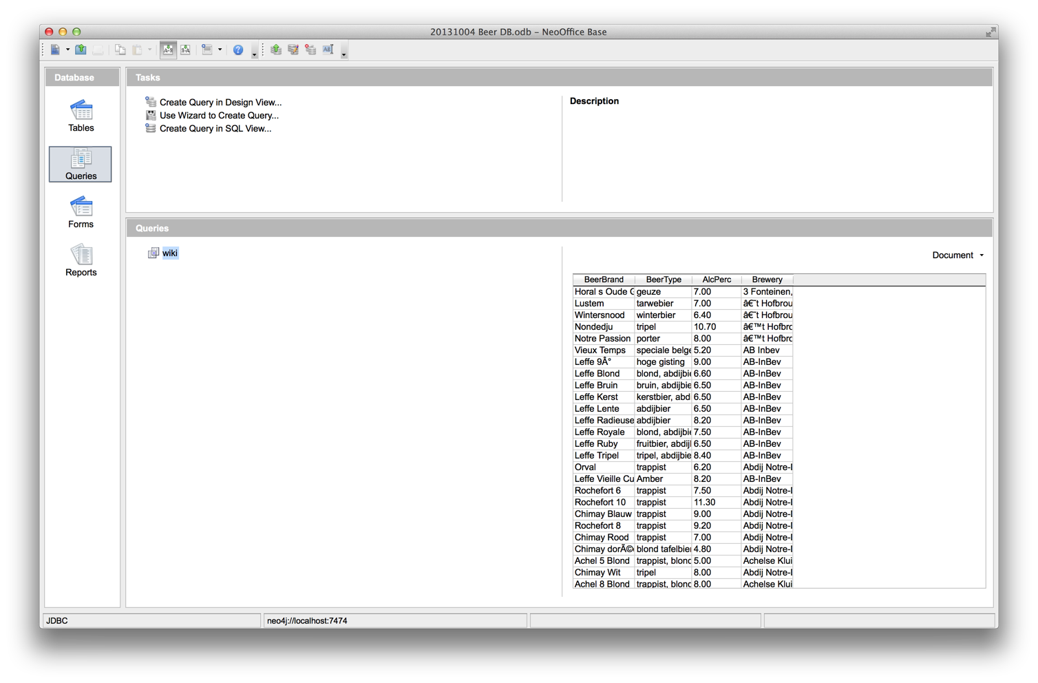
Let’s copy and paste that into the query window, save, give the query a name (in our case "wiki"). Please do remember to push the little “Run SQL Command directly” button , as it will deal with the fact that … we are not running SQL, but indeed using Cypher over the JDBC connector.

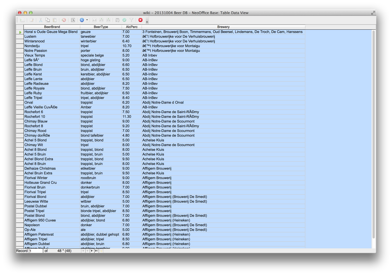
If you then try out the query by double clicking it in the main database window, you should get something very similar to what we are looking for:

So that completes the first step of this exercise. We have our JDBC connectivity set up between the NeoOffice database and neo4j, and a working query to play around with. Now for the spreadsheet part.

Step 2: the spreadsheet step

This second part is actually terribly easy. All we need to do is

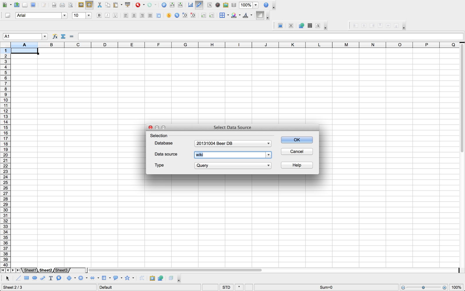
• in the “View” menu of the spreadsheet, we enable the “Data Sources” view. This will then open up a “database” window within the spreadsheet document. Our newly created database - see step 1 above - should now appear in the list of datasources, and our query (in my example, I called the query “wiki”) should also appear as soon as you fold the queries open.
• create a new spreadsheet document
• simply double-clicking the query now gives you access to the query results, within the spreadheet’s top window

The remaining step then, is to copy the query result data into the spreadsheet cells. There’s two ways to do that:

• select the query results in the top right window, position the spreadsheet cursor in the cell that you want the data to go to, and then click the “Data to Text” button
• just grab the query name (top left sub-window) and drag it to the cell that you would like to put it in

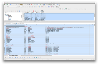
As you can see, we now have the data in a very comparable format to what we started from.

Step 3: the end-user computing step

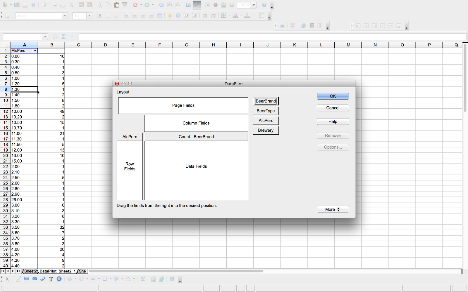
A logical final step then, is to allow the connectivity and spreadsheet integration that we demonstrated above, to do end-user spreadsheet manipulations, like creating a PivotTable/DataPilot sheet that allows me to better understand my dataset.

NeoOffice has a very easy interface to do these things: just start the DataPilot wizard from the “Data” menu in the spreadsheet, and click “Start”.

Then, we reuse the work we did above, and select the registered datasource to base our work of.

The “wiki” query that we executed above, is available under the “query” section, and we can then proceed to the actual construction of the pivottable. We do this by dragging the appropriate “fields” (columns in our cypher resultset) onto the different parts of the pivottable. Once we are ready, we get the following, dynamically composed graph summary table.

I am sure that there are many other things that you can think of doing this way.

Conclusion

I hope that in this post, we have given you a good overview of how you can integrate a traditional software package like NeoOffice/OpenOffice with an advanced, graph-based datastore like neo4j. The possibilities of this connectivity are endless - and we wish you happy hours of data exploration to come.

All the best

Rik