Worldcup Graph!

With the World Cup now in full swing, we really want you to have fun with our amazing Neo4j World Cup Graph Database, that is open for exploration on Heroku. Lot's of cool things to explore - take a look at this video I created to see what kinds of things you can do!



Hope you enjoy!

Rik

Betweenness Centrality: who's the Dolphin Daddy?

Just wrote a graphgist on Betweenness Centrality in a social network of dolphins in the Doubtful Sound, New Zealand. I won't repeat myself here in this blog - but it is pretty fantastic. Thanks to Michael for his help, again.

Graph Local queries - revisited

Recently I had some feedback from Chuck Daniels on my blogpost on Graph Local queries. In the comment, Chuck challenged me in saying that really I should be comparing apples to apples, and that I should make sure that I was applying the same kind of locality.

Basically his question was as follows: once we go from the small dataset to the large one, shouldn't the query that we test performance for also include a richer, more complex pattern. Essentially he wanted me to compare these two queries:

match 

(eqt:EQUIPMENT_TYPE)<-[:IS_OF_TYPE]-(eq:EQUIPMENT)-[:LOCATED_AT]->(ol:OBSERVATION_LOCATION)<-[:OBSERVED_AT_LOCATION]-(o:OBSERVATION {id:1001})

return eqt.name, ol.name, o.id; 

and

match 

(eqt:EQUIPMENT_TYPE)<-[:IS_OF_TYPE]-(eq:EQUIPMENT)-[:LOCATED_AT]->(ol:OBSERVATION_LOCATION)<-[:OBSERVED_AT_LOCATION]-(o:OBSERVATION {id:1001}),

(eq)-[:USED_FOR]->(ot:OBSERVATION_TYPE)<-[:IS_OF_TYPE]-(o)

return eqt.name, ol.name, o.id; 

The second query obviously being a bit more complex, as it adds a few more "hops" to the traversal. 

So lets test this out

I have created a little gist for you to try this yourself. Look at this one for loading the data, and testing the results yourself. We start with an empty database, of course, and load the small dataset first.

Then we run the sample queries (both of them: the easier one AND the more complex one) and create the index on the OBSERVATIONS.

Next up is adding the larger dataset, and running the queries again:

And surprise surprise, the principle of graph locality and index-free adjacency still survived - the queries are still lighting fast. 

Hope this clarifies the point that Chuck raised - and reinforces the fact that graph local queries are GREAT for many different use cases!

All the best

Rik

Dem-O Bones

** UPDATE: I wrote a GraphGist to complement this post as well.

I had so much fun at the Graph Pub tonight in London. It was amazing. Lots of wonderful talks there, and I got to finish it of with my personal Graph Playlist and a LIVE! demo of Dem Bones. Graphs are awesome, and Graphs About Music are even more awesome, at least in my book.

So here is the Graph Playlist for you to contribute to:


Please add it to your Spotify account, if you have one, and start adding songs. Would not mind a #graphplaylist tweet if you do!

Then of course, there was my interpretation of Dem Bones, in a Neo4j database. Here's a little video of it:

You can create the dataset yourself using this gist, and you can query it using the queries in this gist over here. 

Hope you like this as much as I enjoyed creating it.

Cheers

Rik

The power of Graph Local queries

One of the things that I have always found extremely fascinating about Neo4j, and **extremely** annoying about relational database systems, is the way both scale. 

In a relational system, you are often confronted with the fact that queries work fine on your development environment, but then when you go into production and run the same query on a production dataset, it all blows up. As one customer recently put it to me, "the fecal matter would hit the air rotating device". Indeed.

In a graph database, that typically would not happen. Because of the fact that we use index-free adjacency we can pretty much know beforehand that a query that runs fine on a small dataset, will still run fine on a large dataset. The query is local, does not even see the entire graph as it traverses the dataset - it will just traverse that part of the graph that is known to it and accessible from the starting point of the graph query.

Recently, I found a great way to prove that point. Let me take you through that experiment.

Adding a small dataset

I had the opportunity to play with a small dataset of meteorological data recently. It's not very fancy - just a small dataset with a fairly simple model: 

The dataset was small: only containing 148 nodes:

 I created an index on the OBSERVATION nodes to account for a real world scenario:

as we will be using the index to find the starting point of our queries. If I then ran a query that would look for the EQUIPMENT_TYPE of certain OBSERVATIONs (which is a fairly extensive traversal in our small model, this would look like this:

match 

(eqt:EQUIPMENT_TYPE)<-[:IS_OF_TYPE]-(eq:EQUIPMENT)-[:LOCATED_AT]->(ol:OBSERVATION_LOCATION)<-[:OBSERVED_AT_LOCATION]-(o:OBSERVATION {id:1001})return eqt.name, ol.name, o.id; 

On the small dataset that query runs instantaneously: 64 milliseconds.

Then, however, we would like to see if the graph local scalability claim is really true.

Adding half a million observations

What I decided to do was to run a small cypher query that would add a large number of observations to the dataset. 

using periodic commit 10000

match (o:OBSERVATION)-[r:IS_OF_TYPE]->(ot:OBSERVATION_TYPE),

(o)-[s:OBSERVED_AT_LOCATION]->(ol:OBSERVATION_LOCATION)

with range(1,10000) as RANGE,o,r,ot,s,ol

foreach (ran in RANGE | create (ot)<-[:IS_OF_TYPE]-(newobservation:OBSERVATION:DEMO {id: ran+1000000, date: round(rand()*100)+41000 , amount: round(rand())+1 })-[:OBSERVED_AT_LOCATION]->(ol) );

That query actually took 30secs to run on my machine. But it's adding a lot of data as well: 510k nodes, 1020k relationships, 1500k properties and 1020k labels:

Then, we could run the same query as above, but for a different observation, on the new, larger dataset.

Query times at scale: nearly identical

If I now run the same query as above on the larger dataset - but for a different observation - then I am happy to report that the query times are nearly identical:

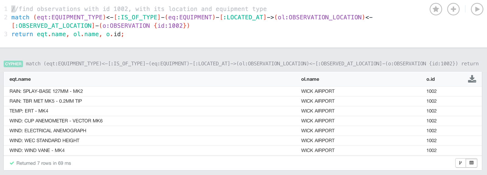
Case in point: the new query runs for about 69 milliseconds.

I truly believe that this is one of the fantastic characteristics of graph databases. Query times typically are not dependant of dataset size - rather dependent of the part of the graph that is traversed, essentially dependant on the result set size.

Hope this was a useful explanation of graph local queries and graph database scalability. I certainly enjoyed it - hope you did too.

Cheers

Rik

Managing Hierarchies in Neo4j - The Video

Had a miserable experience yesterday trying to do a webinar about my "hierarchies" post. All of a sudden the internet in my home office died - in the middle of the f'ing webinar. Terrible. Apologies to all attendees.

Anyway - I decided to record what I wanted to say in this quick video.



Feel free to ask questions in the Comments - I will try to respond as good as I can.

Using Neo4j to Manage and Calculate Hierarchies

I recently had a number of extremely interesting conversations with a company that wants to use Neo4j for managing hierarchical data. This use case is so common, that I decided to write up my findings and experiments and share over here. Hierarchical data is extremely common in many different situations - let's just mention a few:

• organisational data
• Business Continuity Management data
• access control and authentication data (think directory servers like active directory/openldap)
• Product hierarchies (which products are composed of other products)
• Bills of Materials in construction/manufacturing organisations
• etc etc...

Conceptually and mathematically, hierarchies are nothing more than a particular type of graph. Therefore, I would automatically think that finding things in or calculating things over a hierarchy would be a great application for a graph database like neo4j - and that's what this post is about.

Generating a Product Hierarchy

In order to start looking at this, I needed an appropriately sized hierarchy to work with. My normal way of working would be to do something in a spreadsheet and then generate the graph from there - but My dear friend Michael recently wrote a blogpost that inspired me to skip that step. In fact, I can quickly generate a hierarchy myself using Cypher only. Let's talk a look at the following statements:

//Let's create the top of the tree, the PRODUCT
create (n1:PRODUCT {id:1});

//Let's create 100 children of the PRODUCT, COST_GROUPS connected to the top of the tree
match (n1:PRODUCT {id:1})
with range(1,100) as RANGE, n1
foreach (r in RANGE | create (n2:COST_GROUP {id:r})-[:PART_OF {quantity:round(rand()*100)}]->(n1) );

The first query creates the top of the hierarchy, eg. a product. Underneath that we could then create the first level (100 nodes in this example) by iterating through the range and assigning a random identifier to the node and a "quantity" to the "PART_OF" relationship. Semantically, this would mean that the node at Level 1 would be composed of 100 nodes at level 2, using a given quantity of each of the nodes - mentioned on the relationship. In fact, we are building a hierarchy like this one:

So in fact we need to generate another 4 levels underneath the two existing ones, using the same technique as above:

//for every COST_GROUP, let's connect 100 children at a 3rd level, the COST_TYPEs
match (n2:COST_GROUP)
with range(1,100) as RANGE, n2
foreach (r in RANGE | create (n3:COST_TYPE {id:r})-[:PART_OF {quantity:round(rand()*100)}]->(n2) );

//for every COST_TYPE, connect 10 COST_SUBTYPEs 
match (n3:COST_TYPE)
with range(1,10) as RANGE, n3
foreach (r in RANGE | create (n4:COST_SUBTYPE {id:r})-[:PART_OF {quantity:round(rand()*100)}]->(n3) );

//for every COST_SUBTYPE, connect 5 different COSTs
match (n4:COST_SUBTYPE)
with range(1,5) as RANGE, n4
foreach (r in RANGE | create (n5:COST {id:r})-[:PART_OF {quantity:round(rand()*100)}]->(n4) );

So now we already have a graph of 1*100*100*10*5 =500000 nodes. To add the sixth, lowest level of this hierarchy, I actually needed to run three separate queries, as my machine would run out of memory otherwise - the transaction would just be too big:

//for every COST, connect 3 COST_COMPONENTs
match (n5:COST)
create (n6:COST_COMPONENT {id:1,price:round(rand()*1000)})-[:PART_OF {quantity:round(rand()*100)}]->(n5);
match (n5:COST)
create (n6:COST_COMPONENT {id:2,price:round(rand()*1000)})-[:PART_OF {quantity:round(rand()*100)}]->(n5);
match (n5:COST)
create (n6:COST_COMPONENT {id:3,price:round(rand()*1000)})-[:PART_OF {quantity:round(rand()*100)}]->(n5);

As you can see, the sixth level of the hierarchy is a bit different than the ones above, as it includes actual pricing information for the lowest component of the product that we are building. Creating this entire structure on my machine (a 2012 MBP with 8Gbyte of RAM) took about 5minutes, which is not bad in my opinion - it's not a tiny little graph: 2110101 nodes in total.

We can take a look at the browser and see the hierarchy:

So that was already interesting :) ... but now let's see how we can work with these hierarchies, how we can do some interesting queries.

Querying and recalculating the hierarchy - a "graph global" approach

The first scenario that I wanted to explore is to see how fast neo4j would be able to (re)calculate the price of this "complex" (in the sense that it contains millions of parts) product if I would change the price (or the quantity for that matter) of one of the underlying components.  In order to do that, my initial approach was to walk the graph from top to bottom, evaluating the "quantity" property on every relationship, and multiplying that with the price of the COST_COMPONENT at the bottom. Summing all of that would then yield the total price of the product:

//calculating price based on full sweep of the tree
match (n1:PRODUCT {id:1})<-[r1]-(:COST_GROUP)<-[r2]-(:COST_TYPE)<-[r3]-(:COST_SUBTYPE)<-[r4]-(:COST)<-[r5]-(n6:COST_COMPONENT)
return sum(r1.quantity*r2.quantity*r3.quantity*r4.quantity*r5.quantity*n6.price);

One massive advantage of this approach is its simplicity. Cypher is just so great at these types of recursive operations and simplifying the notation for it in a 2 line query. The result comes back in a very reasonable time (43 seconds):

Note that I at first had forgotten to add directions to the relationships, and that this had a massive impact on performance (factor 5 approximately).

What this little test shows, in my humble opinion, and without having done any kind of optimisation of my machine/setup, neo4j is immediately very good at this - it essentially grabs the entire tree, hops along all the 2.1M nodes and relationships to grab the price and the quantities.

Doing some intermediate price calculations

One way of optimizing this kind of operation, of course, is to do some intermediate calculations at every level of the hierarchy. Essentially adding the price at every node as the sum of the prices of the underlying nodes, multiplied by the quantities on the connecting relationships. Let's set that up with the following queries:

//calculate intermediate pricing at the COST level
match (n5:COST)<-[r5]-(n6:COST_COMPONENT)
with n5, sum(r5.quantity*n6.price) as Sum
set n5.price=Sum;

//calculate intermediate pricing at the COST-SUBTYPE level
match (n4:COST_SUBTYPE)<-[r4]-(n5:COST)
with n4,sum(r4.quantity*n5.price) as Sum
set n4.price=Sum;

//calculate intermediate pricing at the COST-TYPE level
match (n3:COST_TYPE)<-[r3]-(n4:COST_SUBTYPE)
with n3,sum(r3.quantity*n4.price) as Sum
set n3.price=Sum;

//calculate intermediate pricing at the COST-GROUP level
match (n2:COST_GROUP)<-[r2]-(n3:COST_TYPE)
with n2,sum(r2.quantity*n3.price) as Sum
set n2.price=Sum;

//calculate intermediate pricing at the PRODUCT level
match (n1:PRODUCT)<-[r1]-(n2:COST_GROUP)
with n1, sum(r1.quantity*n2.price) as Sum
set n1.price=Sum;

Running these queries is really fast:

The advantage of having these intermediate pricing is of course that calculating the price of the product can now be done at every one of the levels. Let's look at two levels: if we use the intermediate pricing at COST-GROUP level, we run this query

//calculate pricing using intermediate pricing levels at the COST-GROUP level
match (n1:PRODUCT {id:1})<-[r1]-(n2:COST_GROUP)
return sum(r1.quantity*n2.price);

and the result is there instantaneously:

Running the same query at the COST-TYPE level takes a bit longer

//calculate pricing using intermediate pricing levels at the COST-TYPE level
match (n1:PRODUCT {id:1})<-[r1]-(n2:COST_GROUP)<-[r2]-(n3:COST_TYPE)
return sum(r1.quantity*r2.quantity*n3.price);

but gives the same result, fortunately:

Interesting. But what would happen if we would change one or more prices of COST_COMPONENTS? How would that affect the hierarchy/graph? Would it perform?

Doing simulations on the hierarchy - recalculating price

If we change something in the price of one of the nodes at the lowest level of the hierarchy, then that would obviously affect the price of the product at the top of the hierarchy. So how can we recalculate price? The "brute force" way is of course to re-run the sweeping query above, and run through the entire hierarchy again. But now that we have the intermediate prices, we can do this much more intelligently.

Essentially what we will do is, when we do the update of the price of the COST_COMPONENT, we will at the same time also update all of the intermediate prices above it. And, consequently, also recalculate the price of the top-level of the hierarchy, the PRODUCT level.

Here's the query that I wrote:

//Changing the price of ONE COST_COMPONENT
match (n6:COST_COMPONENT)
with n6, n6.price as OLDPRICE limit 1
set n6.price = n6.price*10
with n6.price-OLDPRICE as PRICEDIFF,n6
match n6-[r5:PART_OF]->(n5:COST)-[r4:PART_OF]->(n4:COST_SUBTYPE)-[r3:PART_OF]->(n3:COST_TYPE)-[r2:PART_OF]->(n2:COST_GROUP)-[r1:PART_OF]-(n1:PRODUCT)
set n5.price=n5.price+(PRICEDIFF*r5.quantity),
n4.price=n4.price+(PRICEDIFF*r5.quantity*r4.quantity),
n3.price=n3.price+(PRICEDIFF*r5.quantity*r4.quantity*r3.quantity),
n2.price=n2.price+(PRICEDIFF*r5.quantity*r4.quantity*r3.quantity*r2.quantity),
n1.price=n1.price+(PRICEDIFF*r5.quantity*r4.quantity*r3.quantity*r2.quantity*r1.quantity)
return PRICEDIFF, n1.price;

It basically does a couple of things:

• it takes 1 COST_COMPONENT, and extracts the price (OLDPRICE)
• it changes the price of that COST_COMPONENT to *10 as expensive
• it stores the price difference between old and new price in a PRICEDIFF variable
• it then runs through all the levels ABOVE the COST_COMPONENT involved, and changes the intermediate pricing of those nodes. By doing so, we get the new price at the top of the hierarchy.

the result of that changes is also there instantaneously:

We can do the same thing for a hundred COST_COMPONENTS at a time, and still get instantaneous responses. In the following query we increase the pricing of 100 COST_COMPONENTS with 5%:

//Changing the price of ONE HUNDRED COST_COMPONENTS
match (n6:COST_COMPONENT)
with n6, n6.price as OLDPRICE limit 100
set n6.price = round(n6.price*1.05)
with n6.price-OLDPRICE as PRICEDIFF,n6
match n6-[r5:PART_OF]->(n5:COST)-[r4:PART_OF]->(n4:COST_SUBTYPE)-[r3:PART_OF]->(n3:COST_TYPE)-[r2:PART_OF]->(n2:COST_GROUP)-[r1:PART_OF]-(n1:PRODUCT)
set n5.price=n5.price+(PRICEDIFF*r5.quantity),
n4.price=n4.price+(PRICEDIFF*r5.quantity*r4.quantity),
n3.price=n3.price+(PRICEDIFF*r5.quantity*r4.quantity*r3.quantity),
n2.price=n2.price+(PRICEDIFF*r5.quantity*r4.quantity*r3.quantity*r2.quantity),
n1.price=n1.price+(PRICEDIFF*r5.quantity*r4.quantity*r3.quantity*r2.quantity*r1.quantity)
return PRICEDIFF, n1.price;

And the result is there immediately (160ms):

According to the intermediate pricing, the pricing should now be as follows:

If we do another sweeping price calculation then we see that this approach is indeed correct.

Yey!

Conclusion

All of the queries that I wrote for this blogpost are available in the gist over here. If you would run them in your neo4j instance you would be able to create a hierarchy yourself and take a look at the results. Just beware that the hierarchy that I created is quite big, and that some of the transactions involve hundreds of thousands of updates to neo4j in one transaction - and your machine has to be able to do that (mine bombed out on a number of occasions).

Aside from that, I took a away many different things from this weekend exploration of hierarchies in neo4j.

• First of all, without any manipulation of intermediate calculations, neo4j performs fantastically for these types of hierarchical operations. Don't forget, we were looking at a truly large "Product" definition (2.1 millions nodes and relationships for 1 product), and we were recalculating the pricing in under a minute. 
• Secondly, I found that if you would apply the traditional technique of "precalculating" parts of the hierarchy in neo4j (which is what we would always do in relational systems to maintain some kind of performance), the model would become a bit more complicated - but the speed would become AMAZING. 

So there you go - another fantastic use case for neo4j. Anything to do with hierarchies really should be modeled as a graph :) ...

Hope this is useful.

Cheers

Rik