The IDMS EmpDemo - reloaded

A couple of weeks ago, I told the story of the interesting conversation that I had had with Luc Hermans about the similarities between IDMS and Neo4j. Luc gave me access to the EmpDemo dataset that ships with IDMS, and I sort of challenged myself saying that I would love to revisit his 2012 effort to import the data into Neo4j and do some queries on it. Not to see if you could migrate data from IDMS to Neo4j (that would be WAY more complicated, with all the software dependencies, of course), but just to explore the model similarities.

Now, several weeks later, I have something to show you. It's not always very pretty, but here goes :) ...

The IDMS schema file & sequential data

The IDMS input data was essentially structured in two files.

1. The schema file. This file was pretty long and complicated, and describes the structure of the actual data records. Here's an excerpt for the "Coverage" data records:
   

    RECORD NAME IS COVERAGE  
         SHARE STRUCTURE OF RECORD COVERAGE VERSION 100  
         RECORD ID IS 400  
         LOCATION MODE IS VIA EMP-COVERAGE SET  
         WITHIN AREA INS-DEMO-REGION OFFSET 5 PAGES FOR 45 PAGES  
    *+    RECORD NAME SYNONYM IS COVERGE FOR LANGUAGE ASSEMBLER  
    *+    RECORD NAME SYNONYM IS COVRGE FOR LANGUAGE FORTRAN  
    *+    OWNER OF SET COVERAGE-CLAIMS  
    *+      NEXT DBKEY POSITION IS 4  
    *+      PRIOR DBKEY POSITION IS 5  
    *+    MEMBER OF SET EMP-COVERAGE  
    *+      NEXT DBKEY POSITION IS 1  
    *+      PRIOR DBKEY POSITION IS 2  
    *+      OWNER DBKEY POSITION IS 3  
         .  
    *+  02 SELECTION-DATE-0400  
    *+    USAGE IS DISPLAY  
    *+    ELEMENT LENGTH IS 8  
    *+    POSITION IS 1  
    *+    ELEMENT NAME SYNONYM FOR LANGUAGE ASSEMBLER IS COVSELDT  
    *+    ELEMENT NAME SYNONYM FOR LANGUAGE FORTRAN IS CVSLDT  
    *+    .  
   

   As you can see it is all about the "positions" of the data in the file: where does the record start, where do the fields in the record start and end - in the sequential file.
2. The sequential file itself was a lot shorter in this case (it is just a small dataset). The coverage records mentioned above look something like this.
   

    C 00303011978110100000000F003  
     C 00403011975030100000000D004  
     C 00200031977012100000000M002  
     C 00400071978043000000000F004  
     C 00100111980092900000000M001  
     C 00200131981010200000000D002  
     C 00100161978010600000000M001  
   

   As you can see, all it is is a sequence of ASCII numbers that then need to be split up into the different fields, as defined in the schema above. Interesting. 

Unfortunately I can't share the actual files in public - but the above should give you a good idea what I started from.

Struggling with Sequential files - not my forte

Once I grasped these file structures a little bit, I continued to see how I could work with them to create an "importable" format for my Neo4j server. Turned out that was not that easy. I ended up using a two part process:

1. I used a spreadsheet to convert the individual records into structured fields that I could work with. Here's the link to the google doc, if you're interested. Google Sheets has a function called "mid", that allows you to pick contents from a cell's sequential positions:
   
   which was exactly what I needed to do. Once I ficured that out, it was pretty easy to create the nodes in my Neo4j server. But how to extract the relationships???
2. Turns out that I really did not manage to do that. I had to turn to Luc for help, and he basically managed to create a CSV file that used record IDs as the key to establish the relationships. Not pretty - and I still have no clue how he did that (let's just attribute it to the secret art of mainframe wizardry :)), but it did work...

Once I had this all I had to do was to use the structured information in my spreadsheet to generate cypher statements that would allow me to create the graph in Neo4j. That was easy. You can find the statements over here.

Updating the IDMS model to Neo4j

As I already mentioned in the previous blogpost, the similarities between IDMS and Neo4j data models are multiple, but there are also some differences. One of the most striking ones - for me at least - was how IDMS deals with many-to-many cardinalities in the data model. Including these types of relationships in IDMS requires the creation of a separate kind of "record", called a "Junction record". This is a the best explanation that I found over here:

For each many-to-many relationship between two entities, we will almost always identify additional attributes that are not associated with either of the two entities alone, but are associated with the intersection between the two entity types. This intersection is represented by another record type, called junction record type, which has one-to-many relationships with the two entity types. The junction record resolves the many-to-many relationship and implements this many-to-many relationship indirectly. 

Thinking about this some more: junction records are very similar to the relational database concept of a "join table". And as we know, we don't need stuff like that in Neo4j, as you can natively create these kinds of n to m relationships in Neo4j without having to think twice.

So that means that we need to make some updates to the data model, as Luc had already done in his effort. You can clearly see what needs to be done in the figure below:

In the IDMS data model we have three junction records:

• the Emposition: relating the Employees to their jobs
• the Expertise: relating the Employees to their skills
• the Structure: creating a reporting line / managerial relationship between two employees.

So we need to write a Cypher statement that would update the graph accordingly. Here's an example of how I did that for the relationship between Employee and Job:

 //create direct link between employee and job (removing need for "Emposition" juncture record)  
 match (e:Employee)-[r1]-(emp:Emposition)-[r2]-(j:Job)  
 create (e)-[r:JOB_EMPLOYEE]->(j)  
 set r.EmpID=emp.EmpID  
 set r.StartDate=emp.StartDate  
 set r.BonusPercent=emp.BonusPercent  
 set r.SalaryAmount=emp.SalaryAmount  
 set r.OvertimeRate=emp.OvertimeRate  
 set r.EmpositionCode=emp.EmpositionCode  
 set r.CommissionPercent=emp.CommissionPercent  
 set r.FinishDate=emp.FinishDate  
 set r.SalaryGrade=emp.SalaryGrade;  
 //delete the redundant structure  
 //delete r1,r2,emp  

Note that the properties of the junction record (eg. startdate, salary, and others) are now moved from the junction record to a relationship property. Property graphs make relationships equal citizens, don't they! The full update statements that I created are over here. I have put the graph.db folder over here if you want to take if for a spin yourself.

So now, let's do some querying of this dataset with Cypher!

Querying the Reloaded EmpDemo with Cypher

One of the key differences between IDMS and Neo4j seems to be to me that we now have this wonderful query language at our fingertips to explore the network data. IDMS does have some query facilities (using a SQL overlay on top of native IDMS, as I understand it), but it seems to me like the Neo4j approach is a lot more flexible.

Here are some example queries:

 //what's in the dataset  
 match (n)  
 return labels(n), count(n)  
 order by count(n) DESC;  

Gives you the following result:

Or lets do some deeper queries:

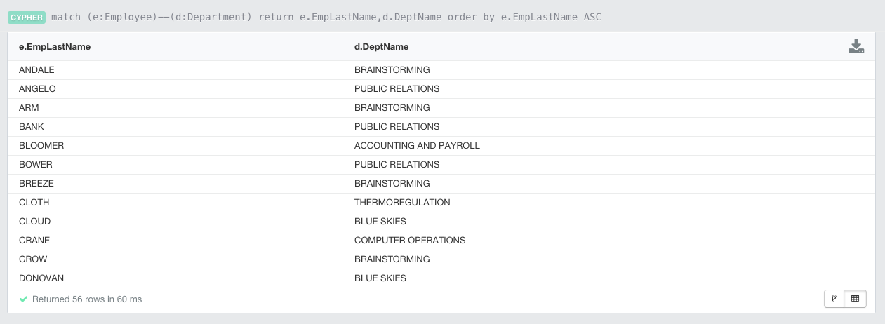
 //Show employee and departments  
 match (e:Employee)--(d:Department)   
 return e.EmpLastName,d.DeptName   
 order by e.EmpLastName ASC  

Gives you:

Of course we can also look at some more graphical representations of our newly reloaded EmpDemo.  To illustrate this, let's look for some shortestpaths between Departments and Skills (bypassing the junction records that we mentioned above):

 //Paths between departments and skills  
 match p=Allshortestpaths((d:Department)-[*]-(s:Skill))   
 return p  
 limit 5;  

This gives you the following result:

Or similarly, let's look for the paths between departments and the different types of claims. This is a bit more interesting, as have different kinds of claims (Dental, Hospital, and Non-Hospital) which currently all have different labels in our data model. We can however, identify them as they all have the same "COVERAGE_CLAIMS" relationship type between the coverage and the different kinds of claims. So that's how the following query was split into two parts:

 //paths between departments and claims  
 match (c)-[ccl:COVERAGE_CLAIMS]-(claim)  
 with c, claim  
 match p=Allshortestpaths((d:Department)-[*]-(c:Coverage))  
 return p,claim  
 limit 1;  

First we look for the Coverage "c" and the Claims "claim" and then we use the AllShortestPaths function to get the links between the departments and the coverage. Running this gives you this (limited to 1 example):

Finally, let's do one more query looking at a broad section of the graph that explores the Employees, Skills and Jobs in one particular department ("EXECUTIVE ADMINISTRATION"). The query is quite simple:

 //Employees, Skills and Jobs in the "Executive Administration" department  
 match p=((d:Department {DeptName:"EXECUTIVE ADMINISTRATION"})--(e:Employee)--(s:Skill)),  
 (e)--(j:Job)  
 return p,j;  

and the result gives you a good view of what goes on in this department:

Obviously you can come up with lots of other queries - just play around with it if you feel like it :)

Wrapping up

This was a very interesting exercise for me. I always knew about the conceptual similarities between Codasyl databases and Neo4j, but I never got to feel it as closely as with this exercise. It feels as if Neo4j - with all its imperfections and limitations that make it probably so much less mature than IDMS today - still does offer some interesting features in terms of flexibility and query capabilities. 

It's as if our industry is going full circle and revisiting the model of the original databases (like IDMS), but enhancing it with some of the expressive query capabilities brought to us by relational databases in the form of SQL. All in all, it does sort of reinforce the image in my mind at least that this really is super interesting and powerful stuff. The network/graph model for data is just fantastic, and if we can make that easily accessible and flexibly usable with tools like Neo4j, the industry can only win. 

Hope this was as useful and interesting for you as it was for me :) ... as always: comments more than welcome.

Cheers

Rik