The power of Graph Local queries

One of the things that I have always found extremely fascinating about Neo4j, and **extremely** annoying about relational database systems, is the way both scale. 

In a relational system, you are often confronted with the fact that queries work fine on your development environment, but then when you go into production and run the same query on a production dataset, it all blows up. As one customer recently put it to me, "the fecal matter would hit the air rotating device". Indeed.

In a graph database, that typically would not happen. Because of the fact that we use index-free adjacency we can pretty much know beforehand that a query that runs fine on a small dataset, will still run fine on a large dataset. The query is local, does not even see the entire graph as it traverses the dataset - it will just traverse that part of the graph that is known to it and accessible from the starting point of the graph query.

Recently, I found a great way to prove that point. Let me take you through that experiment.

Adding a small dataset

I had the opportunity to play with a small dataset of meteorological data recently. It's not very fancy - just a small dataset with a fairly simple model: 

The dataset was small: only containing 148 nodes:

 I created an index on the OBSERVATION nodes to account for a real world scenario:

as we will be using the index to find the starting point of our queries. If I then ran a query that would look for the EQUIPMENT_TYPE of certain OBSERVATIONs (which is a fairly extensive traversal in our small model, this would look like this:

match 

(eqt:EQUIPMENT_TYPE)<-[:IS_OF_TYPE]-(eq:EQUIPMENT)-[:LOCATED_AT]->(ol:OBSERVATION_LOCATION)<-[:OBSERVED_AT_LOCATION]-(o:OBSERVATION {id:1001})return eqt.name, ol.name, o.id; 

On the small dataset that query runs instantaneously: 64 milliseconds.

Then, however, we would like to see if the graph local scalability claim is really true.

Adding half a million observations

What I decided to do was to run a small cypher query that would add a large number of observations to the dataset. 

using periodic commit 10000

match (o:OBSERVATION)-[r:IS_OF_TYPE]->(ot:OBSERVATION_TYPE),

(o)-[s:OBSERVED_AT_LOCATION]->(ol:OBSERVATION_LOCATION)

with range(1,10000) as RANGE,o,r,ot,s,ol

foreach (ran in RANGE | create (ot)<-[:IS_OF_TYPE]-(newobservation:OBSERVATION:DEMO {id: ran+1000000, date: round(rand()*100)+41000 , amount: round(rand())+1 })-[:OBSERVED_AT_LOCATION]->(ol) );

That query actually took 30secs to run on my machine. But it's adding a lot of data as well: 510k nodes, 1020k relationships, 1500k properties and 1020k labels:

Then, we could run the same query as above, but for a different observation, on the new, larger dataset.

Query times at scale: nearly identical

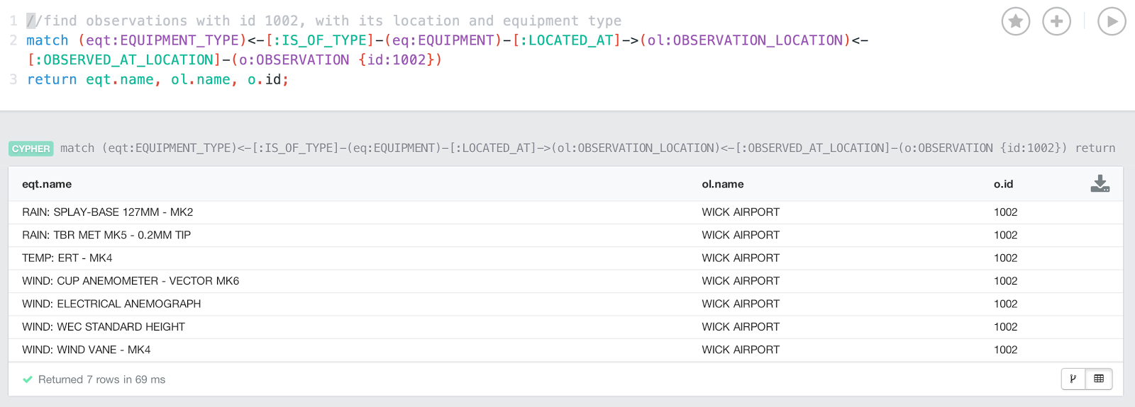
If I now run the same query as above on the larger dataset - but for a different observation - then I am happy to report that the query times are nearly identical:

Case in point: the new query runs for about 69 milliseconds.

I truly believe that this is one of the fantastic characteristics of graph databases. Query times typically are not dependant of dataset size - rather dependent of the part of the graph that is traversed, essentially dependant on the result set size.

Hope this was a useful explanation of graph local queries and graph database scalability. I certainly enjoyed it - hope you did too.

Cheers

Rik

Managing Hierarchies in Neo4j - The Video

Had a miserable experience yesterday trying to do a webinar about my "hierarchies" post. All of a sudden the internet in my home office died - in the middle of the f'ing webinar. Terrible. Apologies to all attendees.

Anyway - I decided to record what I wanted to say in this quick video.



Feel free to ask questions in the Comments - I will try to respond as good as I can.