Summer fun with Musicbrainz: the "real" Six Degrees of Kanye West (part 2/3)

In the first article of this series we talked about our mission to recreate the Six Degrees of Kanye West website in Neo4j - and how we are going to use the (Musicbrainz database)[www.musicbrainz.org] to do that. We have a running postgres database, and now we can start the import of part of the dataset into Neo4j to understand what the infamous Kanye Number of artists would be.

Loading data into Neo4j

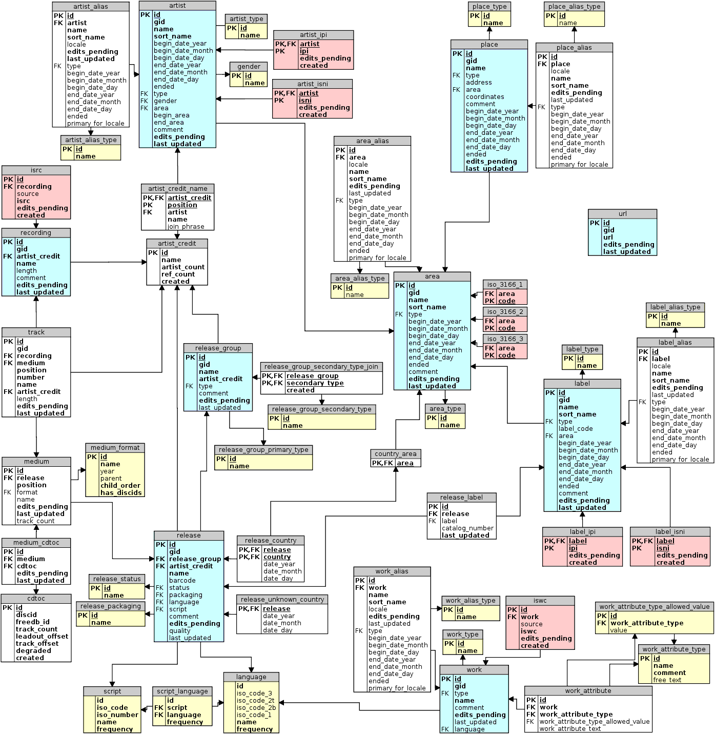
There's lots of different approaches to loadhing the data, but when I started looking at the model in a bit more detail:

 

If we wanted to create our Kanye Number graph out of this, we would need to work that into something like this:

 

To go about that, I started to look into the detail of the schema, and I noticed that the artist and recording tables are linked together to something called the artistcredit. That's what's providing the links between the artists and the recording - the credit. On top of that, as explained on the Musicbrainz website, there are so-called "link tables" that already provide a number of precalculated links between entities. So that lead me to think of a 3 or 4 step import process:

1. import the artists from the artist table;
2. import the recordings from the recording table;
3. import the relationships between artist and recording based on the already present, precalculated link table _l_artist_recording_;
4. last but not least, infer a new set of relationsips between artist and recording, based on the _artist_credit_name_ table.

So let's get cracking with that.

Setting up the JDBC connection

Conceptually, what we are going to do is to setup a JDBC connection between our Neo4j database server, and the Musicbrainz Postgres server. Using that connection, we can use apoc.load.jdbc to pull data from the Postgres server, and work with the resultset of that connection to create and/or update our graph database. Take a look at some of the examples on the website, and read up on the documentation. It's really quite easy to work with, especially once we have the connection set up.

The first thing that we need to do, is to dowload the postgres driver from the postgres site and put the .jar file into the plugins directory of Neo4j server. Then we need to restart the Neo4j server, and load the JDBC driver in cypher, so that apoc.load.jdbc can make use of it.

This does the trick:

call apoc.load.driver('org.postgresql.Driver')

Next, we can start loading data through the JDBC driver into our Neo4j graph database.

Part 1: Load the nodes into the graph

Looking back at the four step process above, we are going to start with the loading of the artist nodes first. Here's how we can do that, at scale, by batching our updates into 10000 record chunks using apoc.periodic.iterate - more info on that is over here.

CALL apoc.periodic.iterate(
  'CALL apoc.load.jdbc("jdbc:postgresql://localhost:5432/musicbrainz_db?user=musicbrainz&password=musicbrainz","artist") yield row',
  'CREATE (a:Artist) SET a += row',
  { batchSize:10000, parallel:true})

Next we can load the recordings in a very similar way:

CALL apoc.periodic.iterate(
  'CALL apoc.load.jdbc("jdbc:postgresql://localhost:5432/musicbrainz_db?user=musicbrainz&password=musicbrainz","recording") yield row',
  'CREATE (r:Recording) SET r += row',
  { batchSize:25000, parallel:true})

Now that we have that, we can start looking at loading the relationships into the graph.

Part 2: Load the relationships into the graph

To add the relationships, not only will we need to look up info from the two tables mentioned above (l_artist_recording and artist_credit_name) in the Postgress database, but we will actually also need to look up corresponding Artist and Recording nodes in the graph to create the links. To speed up these lookups, we will want to create some indexes in the graph database. We do that as follows (note that the syntax for this has actually recently changed, and that we now also have our wonderful now relationship property indexes):

create index for (a:Artist) on (a.id);
create index for (a:Artist) on (a.name);
create fulltext index fulltext_artist_name for (a:Artist) on each [a.name];
create index for (a:Artist) on (a.kanyenr);
create index for (r:Recording) on (r.id);
create index for (r:Recording) on (r.name);
create fulltext index fulltext_recording_name for (r:Recording) on each [r.name];
create index for (r:Recording) on (r.artist_credit);
create index for (ral:RecordingArtistLink) on (ral.entity0);
create index for (ral:RecordingArtistLink) on (ral.entity1);
create index for (acn:ArtistCreditName) on (acn.artist);
create index for (acn:ArtistCreditName) on (acn.artist_credit);
create index for ()-[r:RECORDED]->() on (r.source);

Running that is quick, but not that populating the indexes may take some time, especially with higher volumes:

Now we are ready to proceed.

Create the relationship between artist and recording via the l_artist_recording link table

This will be a three step process:

1. first we actually create temporary nodes in our graph database based on the l_artist_recording table, and call these the (:RecordingArtistLink) nodes.
2. then we create the relationships between (:Recording) and (:Artist) by reading that (:RecordingArtistLink) node and its .entity0 and .entity1 properties. Based on that, we can create the [:RECORDED] relationship, adding the .source property to it as well.
3. then we remive the (:RecordingArtistLink) nodes

The Cypher statement for these operations go like this:

CALL apoc.periodic.iterate(
    'CALL apoc.load.jdbc("jdbc:postgresql://localhost:5432/musicbrainz_db?user=musicbrainz&password=musicbrainz","l_artist_recording") yield row',
    'create (link:RecordingArtistLink) set link += row',
    { batchSize:15000, parallel:true});

CALL apoc.periodic.iterate(
  'match (link:RecordingArtistLink) return link',
  'match (r:Recording), (a:Artist)
  where a.id = link.entity0 and r.id = link.entity1
  merge (a)-[:RECORDED {source:"linktable"}]->(r)',
  { batchSize:5000, parallel:false});

CALL apoc.periodic.iterate(
  'match (link:RecordingArtistLink) return link',
  'delete link',
  { batchSize:25000, parallel:true});

Next, we can do something very similar through the other link table.

Create the relationship between artist and recording via the artist_credit_name table

As we saw in the datamodel above, there is another way to infer the link between artists and recordings, which is through the artist_credit_name table. We will actually apply a very similar, 3-step process here:

1. first we actually create temporary nodes in our graph database based on the artist_credit_name table, and call these the (:ArtistCreditName) nodes.
2. then we create the relationships between (:Recording) and (:Artist) by reading that (:ArtistCreditName) node and its .artist and .artist_credit properties. The .artist identifier corresponds to the .id property on the (:Artist) nodes, and the .artist_credit property corresponds to the .artist_credit property on the (:Recording) nodes. Based on that, we can create the [:RECORDED] relationship, adding the .source property to it as well.
3. then we remive the (:ArtistCreditName) nodes

The Cypher statements for these operations are like this:

CALL apoc.periodic.iterate(
  'CALL apoc.load.jdbc("jdbc:postgresql://localhost:5432/musicbrainz_db?user=musicbrainz&password=musicbrainz","artist_credit_name") yield row',
  'CREATE (acn:ArtistCreditName) SET acn += row',
  { batchSize:15000, parallel:true});
CALL apoc.periodic.iterate(
"match (acn:ArtistCreditName) return acn",
"match (r:Recording), (ar:Artist)
where acn.artist = ar.id and r.artist_credit = acn.artist_credit
merge (r)<-[rec:RECORDED]-(ar)
on create set rec.source='artistcredit'",
{batchSize:10000, parallel:false});
CALL apoc.periodic.iterate(
  'match (link:ArtistCreditName) return link',
  'delete link',
  { batchSize:25000, parallel:true});

Now we actually have a fully functioning Musicbrainz graph, ready to rumble.

And as you can see it's quite a cool and sizeable dataset:

match ()-[r:RECORDED]->() return count(r);

amd

match (n) return distinct labels(n), count(n);

In the next part of this blogpost series, we will explore the querying of this graph together.

Hope this was fun and useful.

Cheers

Rik Van Bruggen

• Twitter
• Blog
• LinkedIn

This post is part of a 3-part series. You can find

• Part 1 over here
• Part 2 over here
• Part 3 over here