Part 1/2: looking at the Web of Belgian Public Companies in Neo4j

Just a few days ago I came across an interesting article on Belgium's premier economic newspaper - (De Tijd, the local equivalent of the Financial Times or the Wall Street Journal) that was over here:

The title of the article is "The Spider's web of publicly traded Belgium", referring to the web of companies, ceo's, chairmen and directors for the 126 public companies that Belgium still has.
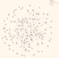
Scrolling down the page, we have this striking visualisation that is included:

The authors: of the visualisation are Michael Sephiha, Thomas Roelens and Maarten Lambrechts - and clearly the did a very good job. But seems the dataset looks so "graphy", it would be kind of natural to try and look at it in Neo4j, right? So that's why these two blog posts are going to be all about

• finding the dataset, and then loading it into Neo4j
• querying the dataset, and finding some new interesting insights (if at all.

So let's get going with that.

Finding the Dataset

So the data of the above visualization had to be coming from somewhere, right? I had a similar experience last year when I was looking for the dataset of the Paris Bataclan Terrorist Attack network, which I wrote about on this blog too. The key of course, is to dig up my HTML-reading skills, and look at the source of the webpage. In Chrome just do view-source:https://multimedia.tijd.be/bestuurders/ and it will show you the page.
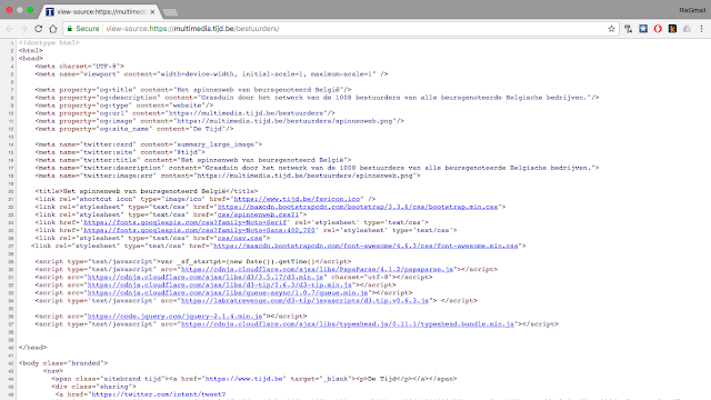
In other browsers, you have similar mechanisms, point is that you can start looking at the source - and very quickly see that the actual visualization is being included by a Javascript file called and referenced by the

<script src="js/spinnenweb.js?1"></script>

tag which is actually located over here. Let's look at that file for a second.

There you very quickly find that the Javascript references two .csv files:

• one for the nodes of the graph: http://multimedia.tijd.be/bestuurders/data/nodesdef.csv
• one for the links or relationships in the graph: http://multimedia.tijd.be/bestuurders/data/linksdef.csv

So now we can think about loading that .csv data into Neo4j. Been there, done that!

Manipulating the data (a little bit)

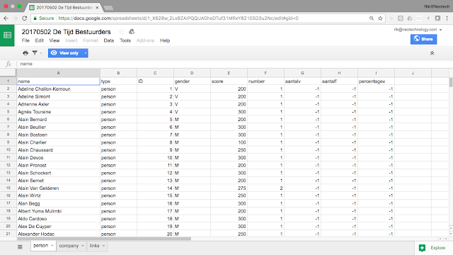
So when I looked at these .csv files in a bit more detail, I quickly noticed that the "nodes" part of the CSV file had two types of entities in it: Persons, and Companies. Both of them had identifiers (the "ID" column), and gender data. The columns also had Dutch headings, so I made a few changes to it and modified it slightly using my goto-data-tool: a Google spreadsheet. I created this specific Google sheet, featuring three worksheets:

1. the Persons sheet. As always, you can make the spreadsheet publicly accessible, and then the Persons sheet can be downloaded as a csv file from a specific URL. 
2. the Companies sheet: can now also be downloaded as a csv file
3. last but not least: the relationships between Persons and Companies can also be downloaded as csv file. This latter file is interesting, as it references different types of relationships. This means we can import the data in different ways, as we will see below.

So now that we have these three slightly modified CSV files, we can proceed and use Cypher's LOAD CSV to import the data into Neo4j. Let's do that.

Loading the data into Neo4j

As you can probably guess, we will do the import in three short steps:

1. add the Person nodes
2. add the Company nodes
3. add the relationships between both of the above.

Let's do that. First we load the person nodes using the following query:

//import the Person nodes 

load csv with headers from"https://docs.google.com/spreadsheets/d/1_X628w_2Lx8ZAIPQQUAGhoDTuf31MRxY821E5D3u2Nc/export?format=csv&id=1_X628w_2Lx8ZAIPQQUAGhoDTuf31MRxY821E5D3u2Nc&gid=0" as personscreate (n:Node:Person)set n = persons;

Two things to note here:

1. we are assigning two Labels to the nodes here. After the import, we will only want the :Person label, but during the relationship import we will want to use the ID of both the Person and the Company nodes to establish these links.
2. with the SET command, I am just assigning all the properties / columns of the csv file to the newly created notes - in other words I am not selecting any of them specifically.

So after a short wait, Neo4j comes back and reports to have imported 1010 nodes:

So once we have done that, we can proceed to import the company nodes. We use this, very similar, import script:

//import the Company nodes 

load csv with headers from"https://docs.google.com/spreadsheets/d/1_X628w_2Lx8ZAIPQQUAGhoDTuf31MRxY821E5D3u2Nc/export?format=csv&id=1_X628w_2Lx8ZAIPQQUAGhoDTuf31MRxY821E5D3u2Nc&gid=2040965723" as companiescreate (n:Node:Company)set n = companies;

And Neo4j reports to have created 127 Companies.

And then last but not least, we finally add the relationship nodes. Now, as mentioned before, the relationship worksheet in the google sheet has a "mandate" column, which basically means that it tells us more about the type of relationship that exists between the two nodes. Now that leaves us with two modelling options:

1. we can create a model that creates a different relationship type for every mandate type, or
2. we can create a model that has one generic "RELATED_TO" relationship type, but then qualifies the relationship with a relationship property.

Both options could be valid, and I have implemented both.

The easier option is to work with the generic relationship type that has a type-property:

//import the relationships 

load csv with headers from "https://docs.google.com/spreadsheets/d/1_X628w_2Lx8ZAIPQQUAGhoDTuf31MRxY821E5D3u2Nc/export?format=csv&id=1_X628w_2Lx8ZAIPQQUAGhoDTuf31MRxY821E5D3u2Nc&gid=773066509" as csvmatch (source:Node {ID: csv.source}), (target:Node {ID: csv.target})create (source)-[:RELATED_TO {type: csv.mandate}]->(target);

This works with standard Cypher, and gives you a quick and easy result.

The second option is to use Neo4j's Awesome Procedures, as standard cypher does not allow you to use a variable relationship type in the LOAD CSV. So, with APOC, we can do that, and create the different relationship types that we mentioned above:

//loading the relationships with APOC: different relationship types 

load csv with headers from "https://docs.google.com/spreadsheets/d/1_X628w_2Lx8ZAIPQQUAGhoDTuf31MRxY821E5D3u2Nc/export?format=csv&id=1_X628w_2Lx8ZAIPQQUAGhoDTuf31MRxY821E5D3u2Nc&gid=773066509" as csvmatch (source:Node {ID: csv.source}), (target:Node {ID: csv.target})CALL apoc.create.relationship(source,csv.mandate,{},target) yield relreturn count(*);

As I said, there's really not that big of a difference - both are possible.

Last but not least, I decided to "colour" the graph a bit more by setting Male and Female labels, so that our lovely Neo4j Browser could assign different blue and pink colours to the graph more easily:

//Colour males and females with new labels 

match (n:Person)where n.gender = "M"set n:Male;match (n:Person)where n.gender = "V"set n:Female;

And lastly, I could also remove the :Node label now - no need for that anymore.

//remove the old labels 

match (n:Node)
remove n:Node;

So this was the result.

We will explore this lovely little graph in the 2nd and final part of this blogpost, soon.

Hope you enjoyed - look forward to hearing your feedback. All of the scripts are on github, you can find them over here.

Cheers

Rik