Graphs for HR Analytics

Yesterday, I had the pleasure of doing a talk at the Brussels Data Science meetup. Some really cool people there, with interesting things to say. My talk was about how graph databases like Neo4j can contribute to HR Analytics. Here are the slides of the talk:

I truly had a lot of fun delivering the talk, but probably even more preparing for it.

My basic points that I wanted to get across where these:

• the HR function could really benefit from a more real world understanding of how information flows in its organization. Information flows through the *real* social network of people in your organization - independent of your "official" hierarchical / matrix-shaped org chart. Therefore it follows logically that it would really benefit the HR function to understand and analyse this information flow, through social network analysis.
• In recruitment, there is a lot to be said to integrate social network information into your recruitment process. This is logical: the social network will tell us something about the social, friendly ties between people - and that will tell us something about how likely they are to form good, performing teams. Several online recruitment platforms are starting to use this - eg. Glassdoor uses Neo4j to store more than 70% of the Facebook sociogram - to really differentiate themselves. They want to suggest and recommend the jobs that people really want.
• In competence management, large organizations can gain a lot by accurately understanding the different competencies that people have / want to have. When putting together multi-disciplinary, often times global teams, this can be a huge time-saver for the project offices chartered to do this. 

For all of these 3 points, a graph database like Neo4j can really help. So I put together a sample dataset that should explain this. Broadly speaking, these queries are in three categories:

1. "Deep queries": these are the types of queries that perform complex pattern matches on the graph. As an example, that would something like: "Find me a friend-of-a-friend of Mike that has the same competencies as Mike, has worked or is working at the same company as Mike, but is currently not working together with Mike." In Neo4j cypher, that would something like this

 match (p1:Person {first_name:"Mike"})-[:HAS_COMPETENCY]->(c:Competency)<-[:HAS_COMPETENCY]-(p2:Person),  
 (p1)-[:WORKED_FOR|:WORKS_FOR]->(co:Company)<-[:WORKED_FOR]-(p2)  
 where not((p1)-[:WORKS_FOR]->(co)<-[:WORKS_FOR]-(p2))  
 with p1,p2,c,co  
 match (p1)-[:FRIEND_OF*2..2]-(p2)  
 return p1.first_name+' '+p1.last_name as Person1, p2.first_name+' '+p2.last_name as Person2, collect(distinct c.name), collect(distinct co.name) as Company;  

2. "Pathfinding queries": this allows you to explore the paths from a certain person to other people - and see how they are connected to eachother. For example, if I wanted to find paths between two people, I could do

 match p=AllShortestPaths((n:Person {first_name:"Mike"})-[*]-(m:Person {first_name:"Brandi"}))  
 return p;  

and get this:

Which is a truly interesting and meaningful representation in many cases.

3. Graph Analysis queries: these are queries that look at some really interesting graph metrics that could help us better understand our HR network. There are some really interesting measures out there, like for example degree centrality, betweenness centrality, pagerank, and triadic closures. Below are some of the queries that implement these (note that I have done some of these also for the Dolphin Social Network). Please be aware that these queries are often times "graph global" queries that can consume quite a bit of time and resources. I would not do this on truly large datasets - but in the HR domain the datasets are often quite limited anyway, and we can consider them as valid examples.

 //Degree centrality  
 match (n:Person)-[r:FRIEND_OF]-(m:Person)  
 return n.first_name, n.last_name, count(r) as DegreeScore  
 order by DegreeScore desc  
 limit 10;  
   
 //Betweenness centrality  
 MATCH p=allShortestPaths((source:Person)-[:FRIEND_OF*]-(target:Person))  
 WHERE id(source) < id(target) and length(p) > 1  
 UNWIND nodes(p)[1..-1] as n  
 RETURN n.first_name, n.last_name, count(*) as betweenness  
 ORDER BY betweenness DESC  
   
 //Missing triadic closures  
 MATCH path1=(p1:Person)-[:FRIEND_OF*2..2]-(p2:Person)  
 where not((p1)-[:FRIEND_OF]-(p2))  
 return path1  
 limit 50;  
   
 //Calculate the pagerank  
 UNWIND range(1,10) AS round  
 MATCH (n:Person)  
 WHERE rand() < 0.1 // 10% probability  
 MATCH (n:Person)-[:FRIEND_OF*..10]->(m:Person)  
 SET m.rank = coalesce(m.rank,0) + 1;  

I am sure you could come up with plenty of other examples. Just to make the point clear, I also made a short movie about it:

The queries for this entire demonstration are on Github. Hope you like it, and that everyone understands that Graph Databases can truly add value in an HR Analytics contect.

Feedback, as always, much appreciated.

Rik

Graph Local queries - revisited

Recently I had some feedback from Chuck Daniels on my blogpost on Graph Local queries. In the comment, Chuck challenged me in saying that really I should be comparing apples to apples, and that I should make sure that I was applying the same kind of locality.

Basically his question was as follows: once we go from the small dataset to the large one, shouldn't the query that we test performance for also include a richer, more complex pattern. Essentially he wanted me to compare these two queries:

match 

(eqt:EQUIPMENT_TYPE)<-[:IS_OF_TYPE]-(eq:EQUIPMENT)-[:LOCATED_AT]->(ol:OBSERVATION_LOCATION)<-[:OBSERVED_AT_LOCATION]-(o:OBSERVATION {id:1001})

return eqt.name, ol.name, o.id; 

and

match 

(eqt:EQUIPMENT_TYPE)<-[:IS_OF_TYPE]-(eq:EQUIPMENT)-[:LOCATED_AT]->(ol:OBSERVATION_LOCATION)<-[:OBSERVED_AT_LOCATION]-(o:OBSERVATION {id:1001}),

(eq)-[:USED_FOR]->(ot:OBSERVATION_TYPE)<-[:IS_OF_TYPE]-(o)

return eqt.name, ol.name, o.id; 

The second query obviously being a bit more complex, as it adds a few more "hops" to the traversal. 

So lets test this out

I have created a little gist for you to try this yourself. Look at this one for loading the data, and testing the results yourself. We start with an empty database, of course, and load the small dataset first.

Then we run the sample queries (both of them: the easier one AND the more complex one) and create the index on the OBSERVATIONS.

Next up is adding the larger dataset, and running the queries again:

And surprise surprise, the principle of graph locality and index-free adjacency still survived - the queries are still lighting fast. 

Hope this clarifies the point that Chuck raised - and reinforces the fact that graph local queries are GREAT for many different use cases!

All the best

Rik

The power of Graph Local queries

One of the things that I have always found extremely fascinating about Neo4j, and **extremely** annoying about relational database systems, is the way both scale. 

In a relational system, you are often confronted with the fact that queries work fine on your development environment, but then when you go into production and run the same query on a production dataset, it all blows up. As one customer recently put it to me, "the fecal matter would hit the air rotating device". Indeed.

In a graph database, that typically would not happen. Because of the fact that we use index-free adjacency we can pretty much know beforehand that a query that runs fine on a small dataset, will still run fine on a large dataset. The query is local, does not even see the entire graph as it traverses the dataset - it will just traverse that part of the graph that is known to it and accessible from the starting point of the graph query.

Recently, I found a great way to prove that point. Let me take you through that experiment.

Adding a small dataset

I had the opportunity to play with a small dataset of meteorological data recently. It's not very fancy - just a small dataset with a fairly simple model: 

The dataset was small: only containing 148 nodes:

 I created an index on the OBSERVATION nodes to account for a real world scenario:

as we will be using the index to find the starting point of our queries. If I then ran a query that would look for the EQUIPMENT_TYPE of certain OBSERVATIONs (which is a fairly extensive traversal in our small model, this would look like this:

match 

(eqt:EQUIPMENT_TYPE)<-[:IS_OF_TYPE]-(eq:EQUIPMENT)-[:LOCATED_AT]->(ol:OBSERVATION_LOCATION)<-[:OBSERVED_AT_LOCATION]-(o:OBSERVATION {id:1001})return eqt.name, ol.name, o.id; 

On the small dataset that query runs instantaneously: 64 milliseconds.

Then, however, we would like to see if the graph local scalability claim is really true.

Adding half a million observations

What I decided to do was to run a small cypher query that would add a large number of observations to the dataset. 

using periodic commit 10000

match (o:OBSERVATION)-[r:IS_OF_TYPE]->(ot:OBSERVATION_TYPE),

(o)-[s:OBSERVED_AT_LOCATION]->(ol:OBSERVATION_LOCATION)

with range(1,10000) as RANGE,o,r,ot,s,ol

foreach (ran in RANGE | create (ot)<-[:IS_OF_TYPE]-(newobservation:OBSERVATION:DEMO {id: ran+1000000, date: round(rand()*100)+41000 , amount: round(rand())+1 })-[:OBSERVED_AT_LOCATION]->(ol) );

That query actually took 30secs to run on my machine. But it's adding a lot of data as well: 510k nodes, 1020k relationships, 1500k properties and 1020k labels:

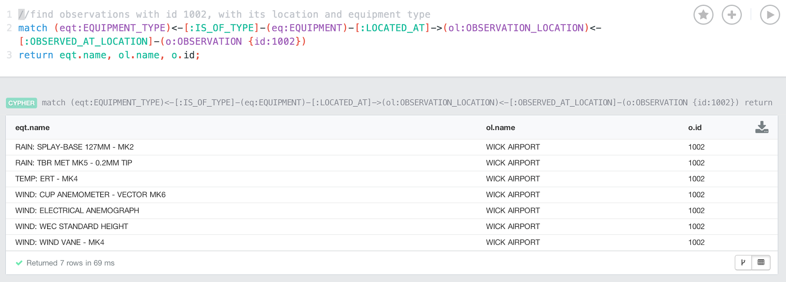
Then, we could run the same query as above, but for a different observation, on the new, larger dataset.

Query times at scale: nearly identical

If I now run the same query as above on the larger dataset - but for a different observation - then I am happy to report that the query times are nearly identical:

Case in point: the new query runs for about 69 milliseconds.

I truly believe that this is one of the fantastic characteristics of graph databases. Query times typically are not dependant of dataset size - rather dependent of the part of the graph that is traversed, essentially dependant on the result set size.

Hope this was a useful explanation of graph local queries and graph database scalability. I certainly enjoyed it - hope you did too.

Cheers

Rik